1. Introducing Image Processing and scikit-image

Jump into digital image structures and learn to process them! Extract data, transform and analyze images using NumPy and Scikit-image. With just a few lines of code, you will convert RGB images to grayscale, get data from them, obtain histograms containing very useful information, and separate objects from the background!

1.1 Make images come alive with scikit-image

Whats the main difference between the images shown below?

Image of coffee next to coins image

These images have been preloaded as coffee_image and coins_image from the scikit-image data module using:

coffee_image = data.coffee()
coins_image = data.coins()

Choose the right answer that best describes the main difference related to color and dimensional structure.

In the console, use the function shape() from NumPy, to obtain the image shape (Height, Width, Dimensions) and find out. NumPy is already imported as np.

Instructions

50 XP

Possible Answers

Both have 3 channels for RGB-3 color representation.
coffee_image has a shape of (303, 384), grayscale. And coins_image (400, 600, 3), RGB-3.
coins_image has a shape of (303, 384), grayscale. And coffee_image (400, 600, 3), RGB-3.
Both are grayscale, with single color dimension.

1.2 Is this gray or full of color?

1.3 RGB to grayscale

In this exercise you will load an image from scikit-image module data and make it grayscale, then compare both of them in the output.

We have preloaded a function show_image(image, title='Image') that displays the image using Matplotlib. You can check more about its parameters using ?show_image() or help(show_image) in the console.

Instructions

100 XP

Import the data and color modules from Scikit image. The first module provides example images, and the second, color transformation functions.
Load the rocket image.
Convert the RGB-3 rocket image to grayscale.

from skimage import data, color

# Load the rocket image
rocket = data.rocket()

# Convert the image to grayscale
gray_scaled_rocket = color.rgb2gray(rocket)

# Show the original image
show_image(rocket, 'Original RGB image')

# Show the grayscale image
show_image(gray_scaled_rocket, 'Grayscale image')

1.4 NumPy for images

1.5 Flipping out

As a prank, someone has turned an image from a photo album of a trip to Seville upside-down and back-to-front! Now, we need to straighten the image, by flipping it.

_Image loaded as flipped_seville._

Using the NumPy methods learned in the course, flip the image horizontally and vertically. Then display the corrected image using the show_image() function.

NumPy is already imported as np.

Instructions 1/3

Flip the image vertically.
Now, flip the vertically-flipped image horizontally.
Show the, now fixed, image.

seville_vertical_flip = np.flipud(flipped_seville)

# Flip the image horizontally
seville_horizontal_flip = np.fliplr(seville_vertical_flip)

# Show the resulting image
show_image(seville_horizontal_flip, 'Seville')

1.6 Histograms

In this exercise, you will analyze the amount of red in the image. To do this, the histogram of the red channel will be computed for the image shown below:

Image loaded as image.

Extracting information from images is a fundamental part of image enhancement. This way you can balance the red and blue to make the image look colder or warmer.

You will use hist() to display the 256 different intensities of the red color. And ravel() to make these color values an array of one flat dimension.

Matplotlib is preloaded as plt and Numpy as np.

Remember that if we want to obtain the green color of an image we would do the following:

green = image[:, :, 1]

Instructions

100 XP

Obtain the red channel using slicing.
Plot the histogram and bins in a range of 256. Don't forget .ravel() for the color channel.

red_channel = image[:, :, 0]

# Plot the red histogram with bins in a range of 256
plt.hist(red_channel.ravel(), bins=256)

# Set title and show
plt.title('Red Histogram')
plt.show()

1.7 Getting started with thresholding

In this exercise, you'll transform a photograph to binary so you can separate the foreground from the background.

To do so, you need to import the required modules, load the image, obtain the optimal thresh value using threshold_otsu() and apply it to the image.

You'll see the resulting binarized image when using the show_image() function, previously explained.

_Image loaded as chess_pieces_image._

Remember we have to turn colored images to grayscale. For that we will use the rgb2gray() function learned in previous video. Which has already been imported for you.

Instructions

100 XP

Instructions

100 XP

Import the otsu threshold function.
Turn the image to grayscale.
Obtain the optimal threshold value of the image.
Apply thresholding to the image.

from skimage.filters import threshold_otsu

# Make the image grayscale using rgb2gray
chess_pieces_image_gray = rgb2gray(chess_pieces_image)

# Obtain the optimal threshold value with otsu
thresh = threshold_otsu(chess_pieces_image_gray)

# Apply thresholding to the image
binary = chess_pieces_image_gray > thresh

# Show the image
show_image(binary, 'Binary image')

1.8 Apply global thresholding

Sometimes, it isn't that obvious to identify the background. If the image background is relatively uniform, then you can use a global threshold value as we practiced before, using threshold_otsu(). However, if there's uneven background illumination, adaptive thresholding threshold_local() (a.k.a. local thresholding) may produce better results.

In this exercise, you will compare both types of thresholding methods (global and local), to find the optimal way to obtain the binary image we need.

_Image loaded as page_image._

Instructions 1/2

50 XP

Import the otsu threshold function, obtain the optimal global thresh value of the image, and apply global thresholding.

from skimage.filters import threshold_otsu

# Obtain the optimal otsu global thresh value
global_thresh = threshold_otsu(page_image)

# Obtain the binary image by applying global thresholding
binary_global = page_image > global_thresh

# Show the binary image obtained
show_image(binary_global, 'Global thresholding')

Import the local threshold function, set block size to 35, obtain the local thresh value, and apply local thresholding.

from skimage.filters import threshold_local

# Set the block size to 35
block_size = 35

# Obtain the optimal local thresholding
local_thresh = threshold_local(page_image, block_size, offset=10)

# Obtain the binary image by applying local thresholding
binary_local = page_image > local_thresh

# Show the binary image
show_image(binary_local, 'Local thresholding')

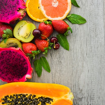
1.9 When the background isn't that obvious

As we saw in the video, not being sure about what thresholding method to use isn't a problem. In fact, scikit-image provides us with a function to check multiple methods and see for ourselves what the best option is. It returns a figure comparing the outputs of different global thresholding methods.

_Image loaded as fruits_image._

You will apply this function to this image, matplotlib.pyplot has been loaded as plt. Remember that you can use try_all_threshold() to try multiple global algorithms.

Instructions

100 XP

Import the try all function.
Import the rgb to gray convertor function.
Turn the fruits image to grayscale.
Use the try all method on the resulting grayscale image.

from skimage.filters import try_all_threshold

# Import the rgb to gray convertor function 
from skimage.color import rgb2gray

# Turn the fruits_image to grayscale
grayscale = rgb2gray(fruits_image)

# Use the try all method on the resulting grayscale image
fig, ax = try_all_threshold(grayscale, verbose=False)

# Show the resulting plots
plt.show()

1.10 Trying other methods

In this exercise, you will decide what type of thresholding is best used to binarize an image of knitting and craft tools. In doing so, you will be able to see the shapes of the objects, from paper hearts to scissors more clearly.

_Image loaded as tools_image._

What type of thresholding would you use judging by the characteristics of the image? Is the background illumination and intensity even or uneven?

Instructions

100 XP

Instructions

100 XP

Import the appropriate thresholding and rgb2gray() functions.
Turn the image to grayscale.
Obtain the optimal thresh.
Obtain the binary image by applying thresholding.

from skimage.filters import threshold_otsu
from skimage.color import rgb2gray

# Turn the image grayscale
gray_tools_image = rgb2gray(tools_image)

# Obtain the optimal thresh
thresh = threshold_otsu(gray_tools_image)

# Obtain the binary image by applying thresholding
binary_image = gray_tools_image > thresh

# Show the resulting binary image
show_image(binary_image, 'Binarized image')

1.11 Apply thresholding

2. Filters, Contrast, Transformation and Morphology

You will learn to detect object shapes using edge detection filters, improve medical images with contrast enhancement and even enlarge pictures to five times its original size! You will also apply morphology to make thresholding more accurate when segmenting images and go to the next level of processing images with Python.

2.1 Jump into filtering

2.2 Edge detection

In this exercise, you'll detect edges in an image by applying the Sobel filter.

Soap pills of heart and rectangle shapes in blue background

Image preloaded as soaps_image.

Theshow_image() function has been already loaded for you.

Let's see if it spots all the figures in the image.

Instructions

100 XP

Import the color module so you can convert the image to grayscale.
Import the sobel() function from filters module.
Make soaps_image grayscale using the appropriate method from the color module.
Apply the sobel edge detection filter on the obtained grayscale image soaps_image_gray.

from skimage import color

# Import the filters module and sobel function
from skimage.filters import sobel

# Make the image grayscale
soaps_image_gray = color.rgb2gray(soaps_image)

# Apply edge detection filter
edge_sobel = sobel(soaps_image_gray)

# Show original and resulting image to compare
show_image(soaps_image, "Original")
show_image(edge_sobel, "Edges with Sobel")

2.3 Blurring to reduce noise

In this exercise you will reduce the sharpness of an image of a building taken during a London trip, through filtering.

Building in Lodon

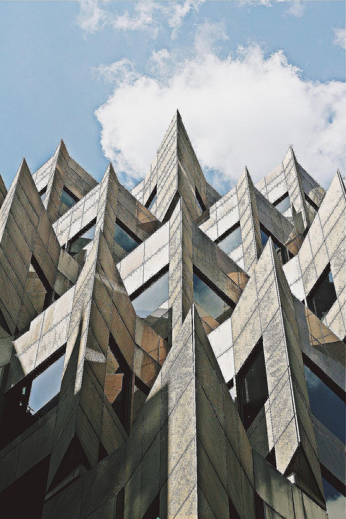
Image loaded as building_image.

Instructions

100 XP

Import the Gaussian filter.
Apply the filter to the building_image, set the multichannel parameter to the correct value.
Show the original building_image and resulting gaussian_image.

from skimage.filters import gaussian

# Apply filter
gaussian_image = gaussian(building_image, multichannel=True)

# Show original and resulting image to compare
show_image(building_image, "Original")
show_image(gaussian_image, "Reduced sharpness Gaussian")

2.4 Contrast enhancement

Black and white clock hanging and moving Histogram of the clock's image

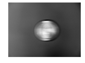
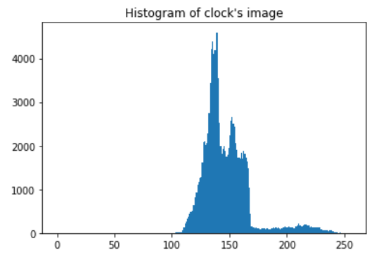
The histogram tell us.

Just as we saw previously, you can calculate the contrast by calculating the range of the pixel intensities i.e. by subtracting the minimum pixel intensity value from the histogram to the maximum one.

You can obtain the maximum pixel intensity of the image by using the np.max() method from NumPy and the minimum with np.min() in the console.

The image has already been loaded as clock_image, NumPy as np and the show_image() function.

Instructions

50 XP

Possible Answers

The contrast is 255 (high contrast).
The contrast is 148.
The contrast is 189.
The contrast is 49 (low contrast).

2.5 What's the contrast of this image?

You are trying to improve the tools of a hospital by pre-processing the X-ray images so that doctors have a higher chance of spotting relevant details. You'll test our code on a chest X-ray image from the National Institutes of Health Chest X-Ray Dataset

X-ray chest image

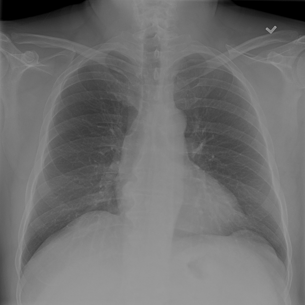
_Image loaded as chest_xray_image._

First, you'll check the histogram of the image and then apply standard histogram equalization to improve the contrast. Remember we obtain the histogram by using the hist() function from Matplotlib, which has been already imported as plt.

Instructions 1/4

25 XP

Import the required Scikit-image module for contrast.

from skimage import exposure

Instructions 2/4

25 XP

Show the histogram from the original x-ray image chest_xray_image, using the hist() function.

from skimage import exposure

# Show original x-ray image and its histogram
show_image(chest_xray_image, 'Original x-ray')

plt.title('Histogram of image')
plt.hist(chest_xray_image.ravel(), bins=256)
plt.show()

Instructions 3/4

25 XP

Use histogram equalization on chest_xray_image to obtain the improved image and load it as xray_image_eq.

from skimage import exposure

# Show original x-ray image and its histogram
show_image(chest_xray_image, 'Original x-ray')

plt.title('Histogram of image')
plt.hist(chest_xray_image.ravel(), bins=256)
plt.show()

# Use histogram equalization to improve the contrast
xray_image_eq =  exposure.equalize_hist(chest_xray_image)

Instructions 4/4

25 XP

Show the resulting improved image xray_image_eq.

from skimage import exposure

# Show original x-ray image and its histogram
show_image(chest_xray_image, 'Original x-ray')

plt.title('Histogram of image')
plt.hist(chest_xray_image.ravel(), bins=256)
plt.show()

# Use histogram equalization to improve the contrast
xray_image_eq =  exposure.equalize_hist(chest_xray_image)

# Show the resulting image
show_image(xray_image_eq, 'Resulting image')

2.6 Medical images

2.7 Aerial image

In this exercise, we will improve the quality of an aerial image of a city. The image has low contrast and therefore we can not distinguish all the elements in it.

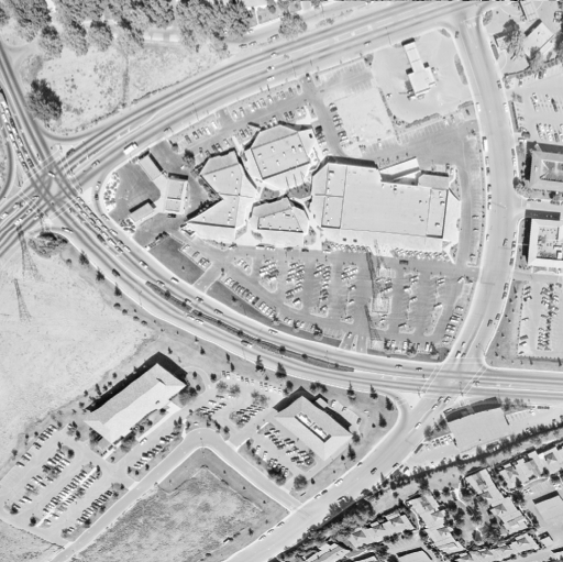
Aerial image, airport taken from the air
_Image loaded as image_aerial._

For this we will use the normal or standard technique of Histogram Equalization.

Instructions

100 XP

Import the required module from scikit-image.
Use the histogram equalization function from the module previously imported.
Show the resulting image.

from skimage import exposure

# Use histogram equalization to improve the contrast
image_eq =  exposure.equalize_hist(image_aerial)

# Show the original and resulting image
show_image(image_aerial, 'Original')
show_image(image_eq, 'Resulting image')

2.8 Let's add some impact and contrast

Have you ever wanted to enhance the contrast of your photos so that they appear more dramatic?

In this exercise, you'll increase the contrast of a cup of coffee. Something you could share with your friends on social media. Don't forget to use #ImageProcessingDatacamp as hashtag!

Even though this is not our Sunday morning coffee cup, you can still apply the same methods to any of our photos.

Cup of coffee

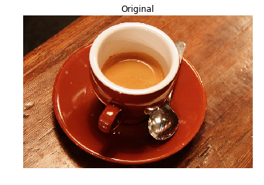
A function called show_image(), that displays an image using Matplotlib, has already been defined. It has the arguments image and title, with title being 'Original' by default.

Instructions

100 XP

Instructions

100 XP

Import the module that includes the Contrast Limited Adaptive Histogram Equalization (CLAHE) function.
Obtain the image you'll work on, with a cup of coffee in it, from the module that holds all the images for testing purposes.
From the previously imported module, call the function to apply the adaptive equalization method on the original image and set the clip limit to 0.03.

from skimage import data, exposure

# Load the image
original_image = data.coffee()

# Apply the adaptive equalization on the original image
adapthist_eq_image = exposure.equalize_adapthist(original_image, clip_limit=0.03)

# Compare the original image to the equalized
show_image(original_image)
show_image(adapthist_eq_image, '#ImageProcessingDatacamp')

2.9 Transformations

2.10 Aliasing, rotating and rescaling

Let's look at the impact of aliasing on images.

Remember that aliasing is an effect that causes different signals, in this case pixels, to become indistinguishable or distorted.

You'll make this cat image upright by rotating it 90 degrees and then rescaling it two times. Once with the anti aliasing filter applied before rescaling and a second time without it, so you can compare them.

Little cute cat
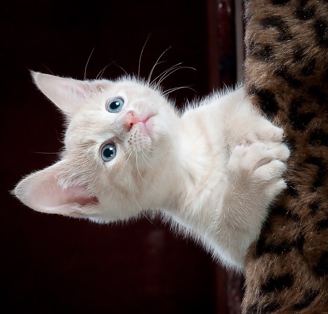
_Image preloaded as image_cat._

Instructions 1/4

25 XP

Import the module and the rotating and rescaling functions.

from skimage.transform import rotate, rescale

Instructions 2/4

25 XP

Rotate the image 90 degrees clockwise.

from skimage.transform import rotate, rescale

# Rotate the image 90 degrees clockwise 
rotated_cat_image = rotate(image_cat, -90)

Instructions 3/4

25 XP

Rescale the cat_image to be 4 times smaller and apply the anti aliasing filter. Set whether or not the image should be treated as multichannel (colored).

from skimage.transform import rotate, rescale

# Rotate the image 90 degrees clockwise 
rotated_cat_image = rotate(image_cat, -90)

# Rescale with anti aliasing
rescaled_with_aa = rescale(rotated_cat_image, 1/4, anti_aliasing=True, multichannel=True)

Instructions 4/4

25 XP

Rescale the rotated_cat_image to be 4 times smaller without applying an anti aliasing filter.

from skimage.transform import rotate, rescale

# Rotate the image 90 degrees clockwise 
rotated_cat_image = rotate(image_cat, -90)

# Rescale with anti aliasing
rescaled_with_aa = rescale(rotated_cat_image, 1/4, anti_aliasing=True, multichannel=True)

# Rescale without anti aliasing
rescaled_without_aa = rescale(rotated_cat_image, 1/4, anti_aliasing=False, multichannel=True)

# Show the resulting images
show_image(rescaled_with_aa, "Transformed with anti aliasing")
show_image(rescaled_without_aa, "Transformed without anti aliasing")

2.11 Enlarging images

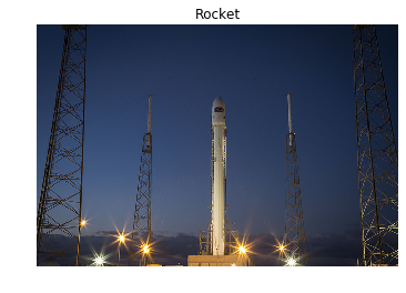
Have you ever tried resizing an image to make it larger? This usually results in loss of quality, with the enlarged image looking blurry.

The good news is that the algorithm used by scikit-image works very well for enlarging images up to a certain point.

In this exercise you'll enlarge an image three times!!

You'll do this by rescaling the image of a rocket, that will be loaded from the data module.

Rocket

Instructions

100 XP

Instructions

100 XP

Import the module and function needed to enlarge images, you'll do this by rescaling.
Import the data module.
Load the rocket() image from data.
Enlarge the rocket_image so it is 3 times bigger, with the anti aliasing filter applied. Make sure to set multichannel to True or you risk your session timing out!

from skimage.transform import rescale

# Import the data module
from skimage import data

# Load the image from data
rocket_image = data.rocket()

# Enlarge the image so it is 3 times bigger
enlarged_rocket_image = rescale(rocket_image, 3, anti_aliasing=True, multichannel=True)

# Show original and resulting image
show_image(rocket_image)
show_image(enlarged_rocket_image, "3 times enlarged image")

2.12 Proportionally resizing

We want to downscale the images of a veterinary blog website so all of them have the same compressed size.

It's important that you do this proportionally, meaning that these are not distorted.

First, you'll try it out for one image so you know what code to test later in the rest of the pictures.

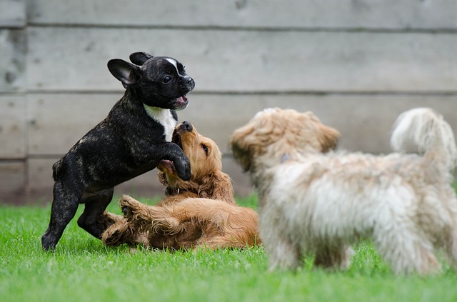
_The image preloaded as dogs_banner._

Remember that by looking at the shape of the image, you can know its width and height.

Instructions

100 XP

Import the module and function to resize.
Set the proportional height and width so it is half the image's height size.
Resize using the calculated proportional height and width.

from skimage.transform import resize

# Set proportional height so its half its size
height = int(dogs_banner.shape[0] / 2)
width = int(dogs_banner.shape[1]  / 2)

# Resize using the calculated proportional height and width
image_resized = resize(dogs_banner, (height, width),
                       anti_aliasing=True)

# Show the original and resized image
show_image(dogs_banner, 'Original')
show_image(image_resized, 'Resized image')

2.13 Morphology

2.14 Handwritten letters

A very interesting use of computer vision in real-life solutions is performing Optical Character Recognition (OCR) to distinguish printed or handwritten text characters inside digital images of physical documents.

Let's try to improve the definition of this handwritten letter so that it's easier to classify.

As we can see it's the letter R, already binary, with some noise in it. It's already loaded as upper_r_image.

Apply the morphological operation that will discard the pixels near the letter boundaries.

Instructions

100 XP

Instructions

100 XP

Import the module from scikit-image.
Apply the morphological operation for eroding away the boundaries of regions of foreground pixels.

from skimage import morphology

# Obtain the eroded shape 
eroded_image_shape = morphology.binary_erosion(upper_r_image) 

# See results
show_image(upper_r_image, 'Original')
show_image(eroded_image_shape, 'Eroded image')

2.15 Improving thresholded image

In this exercise, we'll try to reduce the noise of a thresholded image using the dilation morphological operation.

World map
_Image already loaded as world_image._

This operation, in a way, expands the objects in the image.

Instructions

100 XP

Import the module.
Obtain the binarized and dilated image, from the original image world_image.

from skimage import morphology

# Obtain the dilated image 
dilated_image = morphology.binary_dilation(world_image)

# See results
show_image(world_image, 'Original')
show_image(dilated_image, 'Dilated image')

3. Image restoration, Noise, Segmentation and Contours

So far, you have done some very cool things with your image processing skills! In this chapter, you will apply image restoration to remove objects, logos, text, or damaged areas in pictures! You will also learn how to apply noise, use segmentation to speed up processing, and find elements in images by their contours.

https://projector-video-pdf-converter.datacamp.com/16921/chapter4.pdf#pdfjs.action=download

3.1 Image restoration

3.2 Let's restore a damaged image

In this exercise, we'll restore an image that has missing parts in it, using the inpaint_biharmonic() function.

Small cute puppy

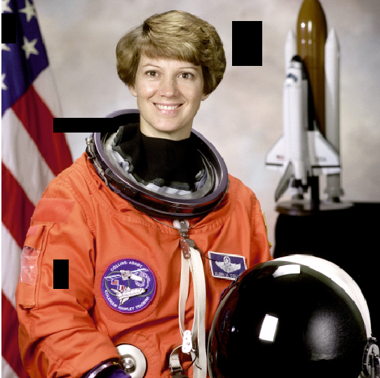
Loaded as defect_image.

We'll work on an image from the data module, obtained by data.astronaut(). Some of the pixels have been replaced with 0s using a binary mask, on purpose, to simulate a damaged image. Replacing pixels with 0s turns them totally black. The defective image is saved as an array called defect_image.

The mask is a black and white image with patches that have the position of the image bits that have been corrupted. We can apply the restoration function on these areas. This mask is preloaded as mask.

Remember that inpainting is the process of reconstructing lost or deteriorated parts of images and videos.

Instructions 1/3

35 XP

Import the inpaint function in the restoration module in scikit-image (skimage).

from skimage.restoration import inpaint

Instructions 2/3

35 XP

Show the defective image using show_image().

from skimage.restoration import inpaint

# Show the defective image
show_image(defect_image, 'Image to restore')

Instructions 3/3

30 XP

Call the correct function from inpaint. Use the corrupted image as the first parameter, then the mask and multichannel boolean.

from skimage.restoration import inpaint

# Show the defective image
show_image(defect_image, 'Image to restore')

# Apply the restoration function to the image using the mask
restored_image = inpaint.inpaint_biharmonic(defect_image, mask, multichannel=True)
show_image(restored_image)

3.3 Removing logos

As we saw in the video, another use of image restoration is removing objects from an scene. In this exercise, we'll remove the Datacamp logo from an image.

_Image loaded as image_with_logo._

You will create and set the mask to be able to erase the logo by inpainting this area.

Remember that when you want to remove an object from an image you can either manually delineate that object or run some image analysis algorithm to find it.

Instructions

100 XP

Instructions

100 XP

Initialize a mask with the same shape as the image, using np.zeros().
In the mask, set the region that will be inpainted to 1 .
Apply inpainting to image_with_logo using the mask.

mask = np.zeros(image_with_logo.shape[:-1])

# Set the pixels where the logo is to 1
mask[210:290, 360:425] = 1

# Apply inpainting to remove the logo
image_logo_removed = inpaint.inpaint_biharmonic(image_with_logo,
                                  mask,
                                  multichannel=True)

# Show the original and logo removed images
show_image(image_with_logo, 'Image with logo')
show_image(image_logo_removed, 'Image with logo removed')

3.4 Noise

In this exercise, we'll practice adding noise to a fruit image.

Various fruits

Image preloaded as fruit_image.

Instructions

100 XP

Import the util module and the random noise function.
Add noise to the image.
Show the original and resulting image.

from skimage.util import random_noise

# Add noise to the image
noisy_image = random_noise(fruit_image)

# Show original and resulting image
show_image(fruit_image, 'Original')
show_image(noisy_image, 'Noisy image')

3.5 Let's make some noise!

We have a noisy image that we want to improve by removing the noise in it.

Small cute puppy

Preloaded as noisy_image.

Use total variation filter denoising to accomplish this.

Instructions

100 XP

Instructions

100 XP

Import the denoise_tv_chambolle function from its module.
Apply total variation filter denoising.
Show the original noisy and the resulting denoised image.

from skimage.restoration import denoise_tv_chambolle

# Apply total variation filter denoising
denoised_image = denoise_tv_chambolle(noisy_image, 
                                      multichannel=True)

# Show the noisy and denoised images
show_image(noisy_image, 'Noisy')
show_image(denoised_image, 'Denoised image')

3.6 Reducing noise

3.7 Reducing noise while preserving edges

In this exercise, you will reduce the noise in this landscape picture.

Landscape of a river

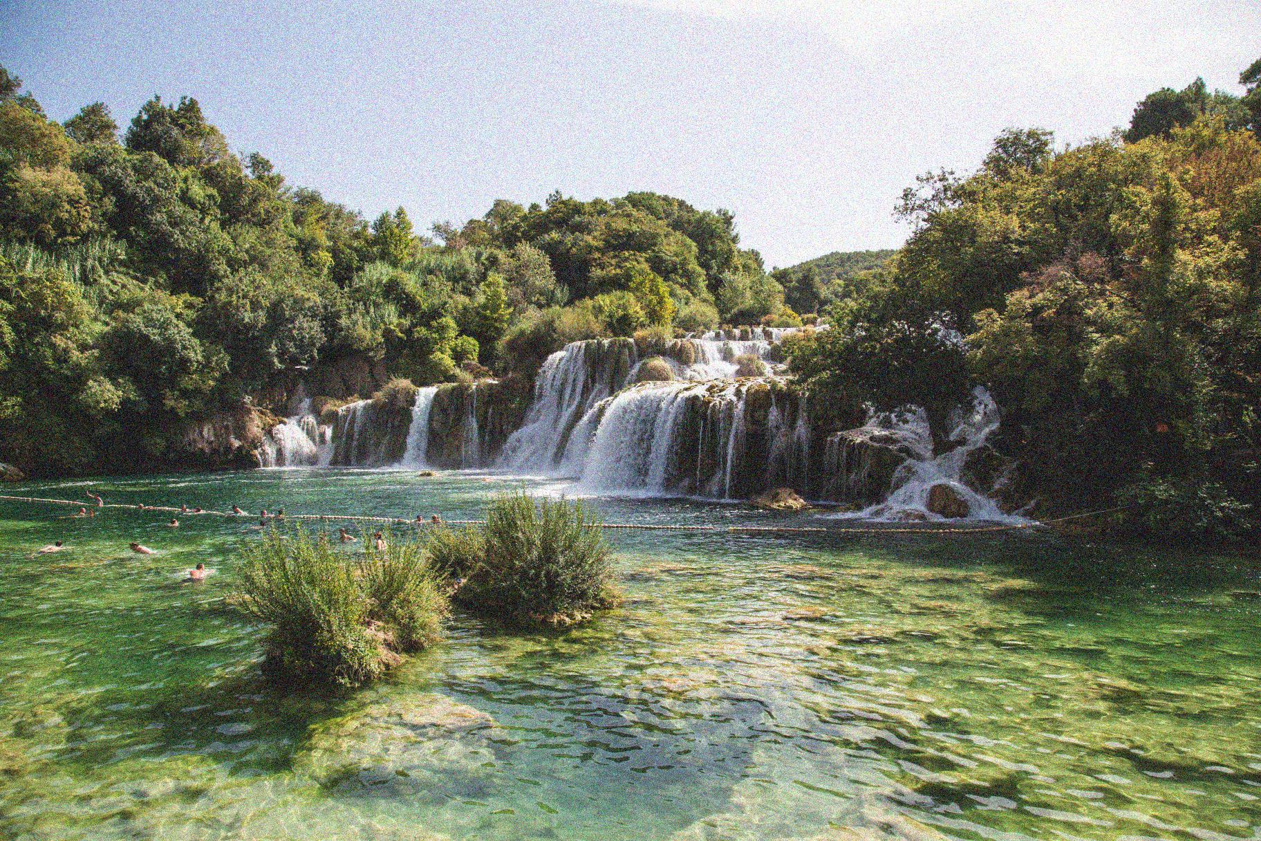
Preloaded as landscape_image.

Since we prefer to preserve the edges in the image, we'll use the bilateral denoising filter.

Instructions

100 XP

Import the denoise_bilateral function from its module.
Apply bilateral filter denoising.
Show the original noisy and the resulting denoised image.

from skimage.restoration import denoise_bilateral

# Apply bilateral filter denoising
denoised_image = denoise_bilateral(landscape_image, 
                                   multichannel=True)

# Show original and resulting images
show_image(landscape_image, 'Noisy image')
show_image(denoised_image, 'Denoised image')

Great! You denoised the image without losing sharpness.
In this case denoise_bilateral() worked well with the default optional parameters.

3.8 Superpixels & segmentation

3.9 Number of pixels

Let's calculate the total number of pixels in this image.

Young woman

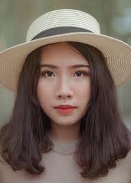
Image preloaded as face_image

The total amount of pixel is its resolution. Given by $ Height × Width $

Use .shape from NumPy which is preloaded as np, in the console to check the width and height of the image.

Instructions

50 XP

Possible Answers

face_image is 191 * 191 = 36,481 pixels
face_image is 265 * 191 = 50,615 pixels
face_image is 1265 * 1191 = 1,506,615 pixels
face_image is 2265 * 2191 = 4,962,615 pixels

In [2]:
face_image.shape
Out[2]:
(265, 191, 3)

Yes! The image is 50,615 pixels in total.

3.10 Superpixel segmentation

In this exercise, you will apply unsupervised segmentation to the same image, before it's passed to a face detection machine learning model.

So you will reduce this image from $265 × 191 = 50,615 pixels$ pixels down to pixels down to $400$ regions.

Already preloaded as face_image.

The show_image() function has been preloaded for you as well.

Instructions

100 XP

Import the slic() function from the segmentation module.
Import the label2rgb() function from the color module.
Obtain the segmentation with 400 regions using slic().
Put segments on top of original image to compare with label2rgb().

from skimage.segmentation import slic

# Import the label2rgb function from color module
from skimage.color import label2rgb

# Obtain the segmentation with 400 regions
segments = slic(face_image,  n_segments= 400)

# Put segments on top of original image to compare
segmented_image = label2rgb(segments, face_image, kind='avg')

# Show the segmented image
show_image(segmented_image, "Segmented image, 400 superpixels")

Awesome work!
You reduced the image from 50,615 pixels to 400 regions! Much more computationally efficient for, for example, face detection machine learning models.

3.11 Finding contours

3.12 Contouring shapes

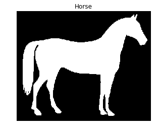
In this exercise we'll find the contour of a horse.

For that we will make use of a binarized image provided by scikit-image in its data module. Binarized images are easier to process when finding contours with this algorithm. Remember that contour finding only supports 2D image arrays.

Once the contour is detected, we will display it together with the original image. That way we can check if our analysis was correct!

show_image_contour(image, contours) is a preloaded function that displays the image with all contours found using Matplotlib.

Shape of a horse in black and white

Remember you can use the find_contours() function from the measure module, by passing the thresholded image and a constant value.

Instructions

100 XP

Instructions

100 XP

Import the data and the module needed for contouring detection.
Obtain the horse image shown in the context area.
Find the contours of the horse image using a constant level value of 0.8.

In this exercise we'll find the contour of a horse.

For that we will make use of a binarized image provided by scikit-image in its data module. Binarized images are easier to process when finding contours with this algorithm. Remember that contour finding only supports 2D image arrays.

Once the contour is detected, we will display it together with the original image. That way we can check if our analysis was correct!

show_image_contour(image, contours) is a preloaded function that displays the image with all contours found using Matplotlib.

Shape of a horse in black and white

Remember you can use the find_contours() function from the measure module, by passing the thresholded image and a constant value.

Instructions

100 XP

Import the data and the module needed for contouring detection.
Obtain the horse image shown in the context area.
Find the contours of the horse image using a constant level value of 0.8.

from skimage import measure, data

# Obtain the horse image
horse_image = data.horse()

# Find the contours with a constant level value of 0.8
contours = measure.find_contours(horse_image, 0.8)

# Shows the image with contours found
show_image_contour(horse_image, contours)

Awesome job! You were able to find the horse contours! In the next exercise you will do some image preparation first and binarize the image yourself before finding the contours.

3.13 Find contours of an image that is not binary

Let's work a bit more on how to prepare an image to be able to find its contours and extract information from it.

We'll process an image of two purple dice loaded as image_dice and determine what number was rolled for each dice.

Purple dice

In this case, the image is not grayscale or binary yet. This means we need to perform some image pre-processing steps before looking for the contours. First, we'll transform the image to a 2D array grayscale image and next apply thresholding. Finally, the contours are displayed together with the original image.

color, measure and filters modules are already imported so you can use the functions to find contours and apply thresholding.

We also import the io module to load the image_dice from local memory, using imread. Read more here.

Instructions 1/4

35 XP

Transform the image to grayscale using rgb2gray().

image_dice = color.rgb2gray(image_dice)

Instructions 2/4

35 XP

Obtain the optimal threshold value for the image and set it as thresh.

image_dice = color.rgb2gray(image_dice)

# Obtain the optimal thresh value
thresh = filters.threshold_otsu(image_dice)

Instructions 3/4

0 XP

Apply thresholding to the image once you have the optimal threshold value thresh, using the corresponding operator.

image_dice = color.rgb2gray(image_dice)

# Obtain the optimal thresh value
thresh = filters.threshold_otsu(image_dice)

# Apply thresholding
binary = image_dice > thresh

Instructions 4/4

30 XP

Apply the corresponding function to obtain the contours and use a value level of 0.8.

image_dice = color.rgb2gray(image_dice)

# Obtain the optimal thresh value
thresh = filters.threshold_otsu(image_dice)

# Apply thresholding
binary = image_dice > thresh

# Find contours at a constant value of 0.8
contours = measure.find_contours(binary, 0.8)

# Show the image
show_image_contour(image_dice, contours)

Great work! You made the image a 2D array by slicing, applied thresholding and succesfully found the contour. Now you can apply it to any image you work on in the future.

3.14 Count the dots in a dice's image

Now we have found the contours, we can extract information from it.

In the previous exercise, we prepared a purple dices image to find its contours:

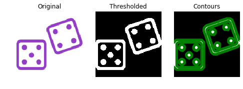
3 images showing the steps to find contours

This time we'll determine what number was rolled for the dice, by counting the dots in the image.

The contours found in the previous exercise are preloaded as contours.

Create a list with all contour's shapes as shape_contours. You can see all the contours shapes by calling shape_contours in the console, once you have created it.

Check that most of the contours aren't bigger in size than 50. If you count them, they are the exact number of dots in the image.

show_image_contour(image, contours) is a preloaded function that displays the image with all contours found using Matplotlib.

Instructions

100 XP

Make shape_contours be a list with all contour shapes of contours.
Set max_dots_shape to 50.
Set the shape condition of the contours to be the maximum shape size of the dots max_dots_shape.
Print the dice's number.

shape_contours = [cnt.shape[0] for cnt in contours]

# Set 50 as the maximum size of the dots shape
max_dots_shape = 50

# Count dots in contours excluding bigger than dots size
dots_contours = [cnt for cnt in contours if np.shape(cnt)[0] < max_dots_shape]

# Shows all contours found 
show_image_contour(binary, contours)

# Print the dice's number
print("Dice's dots number: {}. ".format(len(dots_contours)))

<script.py> output:
    Dice's dots number: 9.

Great work! You calculated the dice's number in the image by classifing its contours.

4. Advanced Operations, Detecting Faces and Features

After completing this chapter, you will have a deeper knowledge of image processing as you will be able to detect edges, corners, and even faces! You will learn how to detect not just front faces but also face profiles, cat, or dogs. You will apply your skills to more complex real-world applications. Learn to master several widely used image processing techniques with very few lines of code!

link PDF

4.1 Finding the edges with Canny

4.2 Edges

In this exercise you will identify the shapes in a grapefruit image by detecting the edges, using the Canny algorithm.

Grapefruits

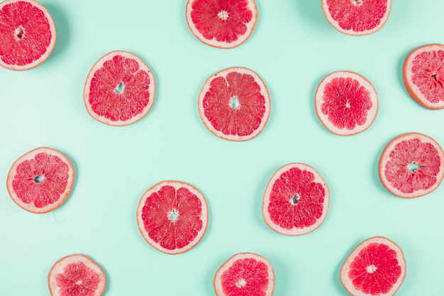
Image preloaded as grapefruit.

The color module has already been preloaded for you.

Instructions

100 XP

Import the canny edge detector from the feature module.
Convert the image to grayscale, using the method from the color module used in previous chapters.
Apply the canny edge detector to the grapefruit image.

from skimage.feature import canny

# Convert image to grayscale
grapefruit =  color.rgb2gray(grapefruit)

# Apply canny edge detector
canny_edges = canny(grapefruit)

# Show resulting image
show_image(canny_edges, "Edges with Canny")

You can see the shapes and details of the grapefruits of the original image being highlighted.

4.3 Less edgy

Let's now try to spot just the outer shape of the grapefruits, the circles. You can do this by applying a more intense Gaussian filter to first make the image smoother. This can be achieved by specifying a bigger sigma in the canny function.

In this exercise, you'll experiment with sigma values of the canny() function.

Grapefruits

Image preloaded as grapefruit.

The show_image has already been preloaded.

Instructions 1/3

35 XP

Instructions 1/3

35 XP

Apply the canny edge detector to the grapefruit image with a sigma of 1.8.

canny_edges = canny(grapefruit, sigma=1.8)

Apply the canny edge detector to the grapefruit image with a sigma of 2.2.

edges_1_8 = canny(grapefruit, sigma=1.8)

# Apply canny edge detector with a sigma of 2.2
edges_2_2 = canny(grapefruit, 2.2)

Show the resulting images.

edges_1_8 = canny(grapefruit, sigma=1.8)

# Apply canny edge detector with a sigma of 2.2
edges_2_2 = canny(grapefruit, sigma=2.2)

# Show resulting images
show_image(edges_1_8, "Sigma of 1.8")
show_image(edges_2_2, "Sigma of 2.2")

The bigger the sigma value, the less edges are detected because of the gaussian filter pre applied.

4.4 Right around the corner

In this exercise, you will detect the corners of a building using the Harris corner detector.

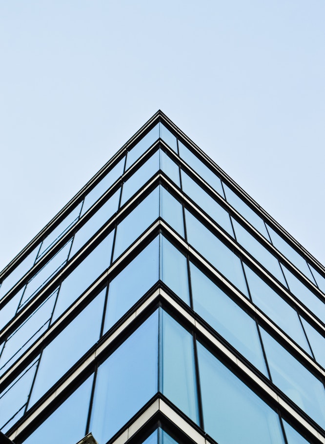
Building from a bottom perspective

Image preloaded as building_image.

The functions show_image() and show_image_with_corners() have already been preloaded for you. As well as the color module for converting images to grayscale.

Instructions

100 XP

Import the corner_harris() function from the feature module.
Convert the building_image to grayscale.
Apply the harris detector to obtain the measure response image with the possible corners.
Find the peaks of the corners.

from skimage.feature import corner_harris, corner_peaks

# Convert image from RGB-3 to grayscale
building_image_gray = color.rgb2gray(building_image)

# Apply the detector  to measure the possible corners
measure_image = corner_harris(building_image_gray)

# Find the peaks of the corners using the Harris detector
coords = corner_peaks(measure_image, min_distance=2)

# Show original and resulting image with corners detected
show_image(building_image, "Original")
show_image_with_corners(building_image, coords)

Great! You made the Harris algorithm work fine.

$image.png$

4.5 Perspective

In this exercise, you will test what happens when you set the minimum distance between corner peaks to be a higher number. Remember you do this with the min_distance attribute parameter of the corner_peaks() function.

Building from a bottom perspective

Image preloaded as building_image.

The functions show_image(), show_image_with_corners() and required packages have already been preloaded for you. As well as all the previous code for finding the corners. The Harris measure response image obtained with corner_harris() is preloaded as measure_image.

Instructions 1/3

35 XP

Find the peaks of the corners with a minimum distance of 2 pixels.

Take Hint (-10 XP)
Find the peaks of the corners with a minimum distance of 40 pixels.
Show original and resulting image with corners detected.

def show_image_with_corners(image, coords, title="Corners detected"):
    plt.imshow(image, interpolation='nearest', cmap='gray')
    plt.title(title)
    plt.plot(coords[:, 1], coords[:, 0], '+r', markersize=15)
    plt.axis('off')
    plt.show()
    plt.close()

coords_w_min_2 = corner_peaks(measure_image, min_distance=2)
print("With a min_distance set to 2, we detect a total", len(coords_w_min_2), "corners in the image.")

# Find the peaks with a min distance of 40 pixels
coords_w_min_40 = corner_peaks(measure_image, min_distance=40)
print("With a min_distance set to 40, we detect a total", len(coords_w_min_40), "corners in the image.")

# Show original and resulting image with corners detected
show_image_with_corners(building_image, coords_w_min_2, "Corners detected with 2 px of min_distance")
show_image_with_corners(building_image, coords_w_min_40, "Corners detected with 40 px of min_distance")

Well done! With a 40-pixel distance between the corners there are a lot less corners than with 2 pixels.

4.6 Less corners

4.7 Face detection

4.8 Is someone there?

In this exercise, you will check whether or not there is a person present in an image taken at night.

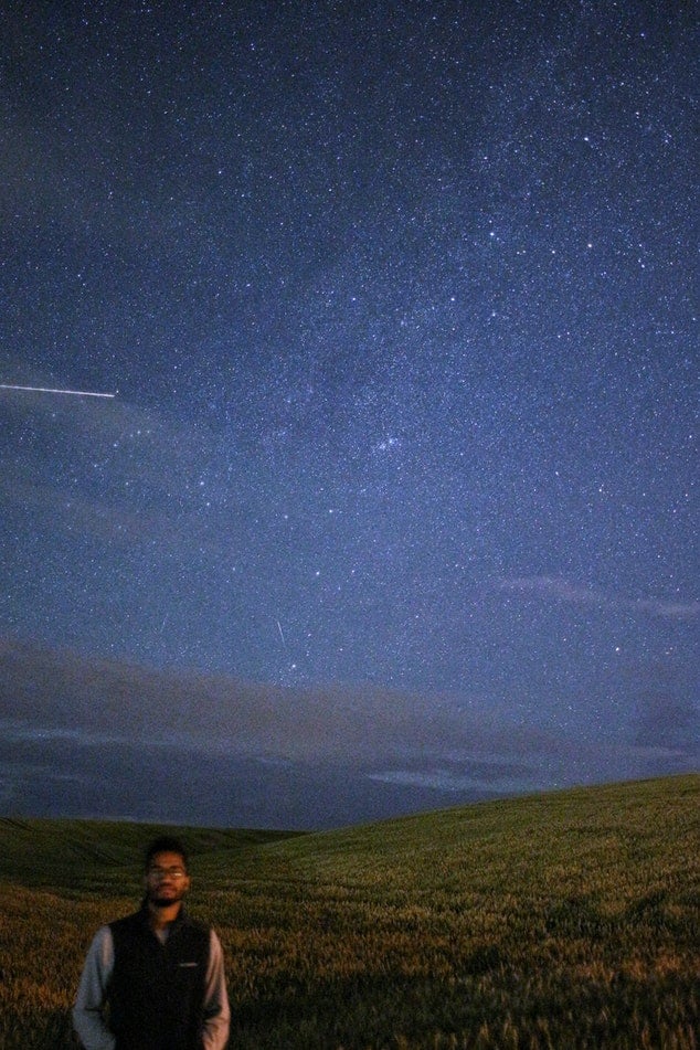
LAndscape of starry night with a young man in the left bottom corner

Image preloaded as night_image.

The Cascade of classifiers class from feature module has been already imported. The same is true for the show_detected_face() function, that is used to display the face marked in the image and crop so it can be shown separately.

Instructions

100 XP

Instructions

100 XP

Load the trained file from the data module.
Initialize the detector cascade with the trained file.
Detect the faces in the image, setting the minimum size of the searching window to 10 pixels and 200 pixels for the maximum.

def show_detected_face(result, detected, title="Face image"):
    plt.figure()
    plt.imshow(result)
    img_desc = plt.gca()
    plt.set_cmap('gray')
    plt.title(title)
    plt.axis('off')

    for patch in detected:
        
        img_desc.add_patch(
            patches.Rectangle(
                (patch['c'], patch['r']),
                patch['width'],
                patch['height'],
                fill=False,
                color='r',
                linewidth=2)
        )
    plt.show()
    crop_face(result, detected)

def crop_face(result, detected, title="Face detected"):
    for d in detected:
        print(d)
        rostro= result[d['r']:d['r']+d['width'], d['c']:d['c']+d['height']]
    
        plt.figure(figsize=(8, 6))
        plt.imshow(rostro)    
        plt.title(title)
        plt.axis('off')
        plt.show()

trained_file = data.lbp_frontal_face_cascade_filename()

# Initialize the detector cascade
detector = Cascade(trained_file)

# Detect faces with min and max size of searching window
detected = detector.detect_multi_scale(img = night_image,
                                       scale_factor=1.2,
                                       step_ratio=1,
                                       min_size=(10,10),
                                       max_size=(200,200))

# Show the detected faces
show_detected_face(night_image, detected)

The detector found the face even when it's very small and pixelated. Note though that you would ideally want a well-illuminated image for detecting faces.

4.9 Multiple faces

In this exercise, you will detect multiple faces in an image and show them individually. Think of this as a way to create a dataset of your own friends' faces!

A group of 7 friends

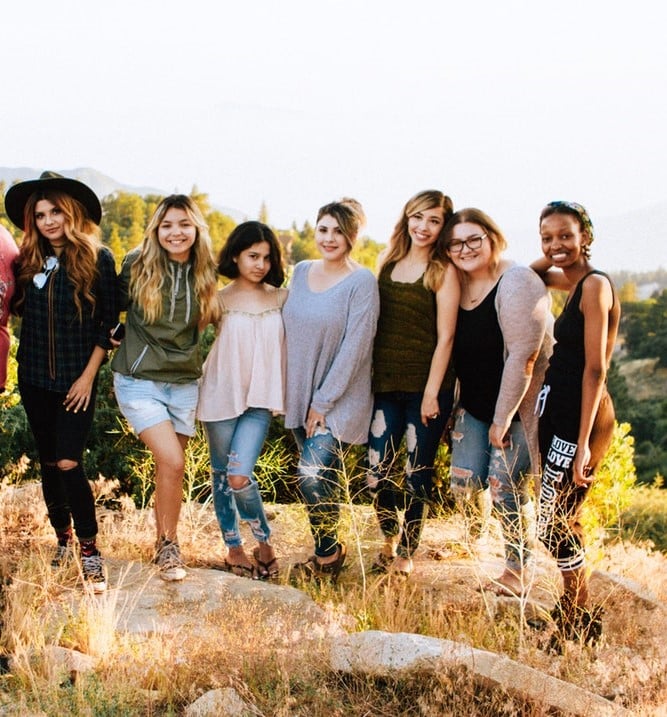
Image preloaded as friends_image.

The Cascade of classifiers class from feature module has already been imported, as well as the show_detected_face() function which is used to display the face marked in the image and crop it so it can be shown separately.

Instructions

100 XP

Load the trained file .lbp_frontal_face_cascade_filename(). from the data module.
Initialize the detector cascade with trained file.
Detect the faces in the image, setting a scale_factor of 1.2 and step_ratio of 1.

trained_file = data.lbp_frontal_face_cascade_filename()

# Initialize the detector cascade
detector = Cascade(trained_file)

# Detect faces with scale factor to 1.2 and step ratio to 1
detected = detector.detect_multi_scale(img=friends_image,
                                       scale_factor=1.2,
                                       step_ratio=1,
                                       min_size=(10, 10),
                                       max_size=(200, 200))
# Show the detected faces
show_detected_face(friends_image, detected)

Wow! The detector gave you a list with all the detected faces. Can you think about what you can use this for?

4.10 Segmentation and face detection

Previously, you learned how to make processes more computationally efficient with unsupervised superpixel segmentation. In this exercise, you'll do just that!

Using the slic() function for segmentation, pre-process the image before passing it to the face detector.

Young woman selfie

Image preloaded as profile_image.

The Cascade class, the slic() function from segmentation module, and the show_detected_face() function for visualization have already been imported. The detector is already initialized and ready to use as detector.

Instructions

100 XP

Apply superpixel segmentation and obtain the segments a.k.a. labels using slic().
Obtain the segmented image using label2rgb(), passing the segments and profile_image.
Detect the faces, using the detector with multi scale method.

segments = slic(profile_image,  n_segments= 100)

# Obtain segmented image using label2rgb
segmented_image = label2rgb(segments, profile_image, kind='avg')

# Detect the faces with multi scale method
detected = detector.detect_multi_scale(img=segmented_image, 
                                       scale_factor=1.2, 
                                       step_ratio=1, 
                                       min_size=(10, 10), max_size=(1000, 1000))

# Show the detected faces
show_detected_face(segmented_image, detected)

Hurray! You applied segementation to the image before passing it to the face detector and it's finding the face even when the image is relatively large. This time you used 1000 by 1000 pixels as the maximum size of the searching window because the face in this case was indeed rather larger in comparison to the image.

4.11 Real-world applications

4.12 Privacy protection

Let's look at a real-world application of what you have learned in the course.

In this exercise, you will detect human faces in the image and for the sake of privacy, you will anonymize data by blurring people's faces in the image automatically.

Group band walking

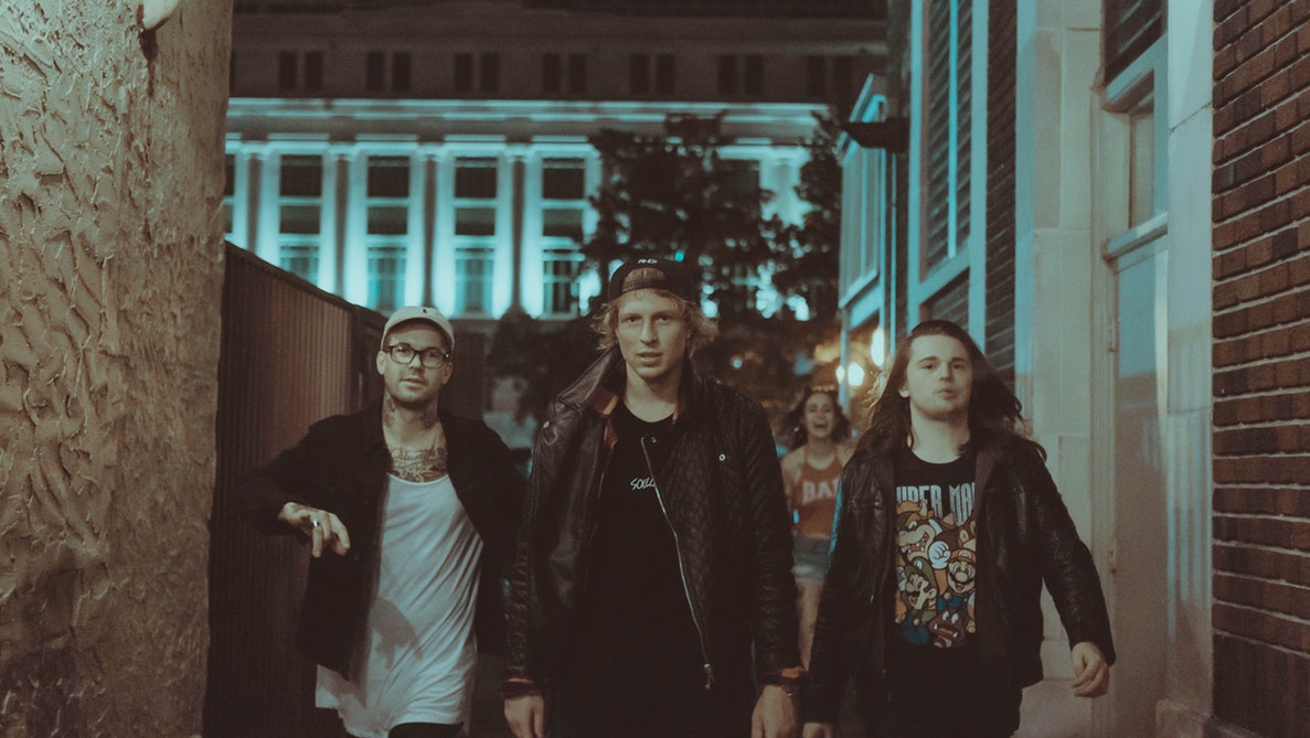
Image preloaded as group_image.

You can use the gaussian filter for the blurriness.

The face detector is ready to use as detector and all packages needed have been imported.

Instructions

100 XP

Detect the faces in the image using the detector, set the minimum size of the searching window to 10 by 10 pixels.
Go through each detected face with a for loop.
Apply a gaussian filter to detect and blur faces, using a sigma of 8.

detected = detector.detect_multi_scale(img=group_image, 
                                       scale_factor=1.2, step_ratio=1, 
                                       min_size=(10, 10), max_size=(100, 100))
# For each detected face
for d in detected:  
    # Obtain the face rectangle from detected coordinates
    face = getFaceRectangle(d)
    
    # Apply gaussian filter to extracted face
    blurred_face = gaussian(face, multichannel=True, sigma = 8)
    
    # Merge this blurry face to our final image and show it
    resulting_image = mergeBlurryFace(group_image, blurred_face) 
show_image(resulting_image, "Blurred faces")

Awesome work! You solved this important issue by applying what you have learned in the course.

4.13 Help Sally restore her graduation photo

You are going to combine all the knowledge you acquired throughout the course to complete a final challenge: reconstructing a very damaged photo.

Help Sally restore her favorite portrait which was damaged by noise, distortion, and missing information due to a breach in her laptop.

Sally damaged picture

Sally's damaged portrait is already loaded as damaged_image.

You will be fixing the problems of this image by:

Rotating it to be uprightusing rotate()
Applying noise reduction with denoise_tv_chambolle()
Reconstructing the damaged parts with inpaint_biharmonic() from the inpaint module.

show_image() is already preloaded.

Instructions

100 XP

Instructions

100 XP

Import the necessary module to apply restoration on the image.
Rotate the image by calling the function rotate().
Use the chambolle algorithm to remove the noise from the image.
With the mask provided, use the biharmonic method to restore the missing parts of the image and obtain the final image.

def get_mask(image):
    # Create mask with three defect regions: left, middle, right respectively
    mask_for_solution = np.zeros(image.shape[:-1])
    mask_for_solution[450:475, 470:495] = 1
    mask_for_solution[320:355, 140:175] = 1
    mask_for_solution[130:155, 345:370] = 1
    return mask_for_solution

from skimage.restoration import denoise_tv_chambolle, inpaint
from skimage import transform

# Transform the image so it's not rotated
upright_img = transform.rotate(damaged_image, 20)

# Remove noise from the image, using the chambolle method
upright_img_without_noise = denoise_tv_chambolle(upright_img,weight=0.1, multichannel=True)

# Reconstruct the image missing parts
mask = get_mask(upright_img)
result = inpaint.inpaint_biharmonic(upright_img_without_noise, mask, multichannel=True)

show_image(result)

Great work! You have learned a lot about image processing methods and algorithms: You performed rotation, removed annoying noise, and fixed the missing pixels of the damaged image. Sally is happy and proud of you!