
This is the memo of the 3rd course (5 courses in all) of ‘Machine Learning with Python’ skill track.
You can find the original course HERE .
#### KNN classification
In this exercise you’ll explore a subset of the
Large Movie Review Dataset
. The variables
X_train
,
X_test
,
y_train
, and
y_test
are already loaded into the environment. The
X
variables contain features based on the words in the movie reviews, and the
y
variables contain labels for whether the review sentiment is positive (+1) or negative (-1).
This course touches on a lot of concepts you may have forgotten, so if you ever need a quick refresher, download the Scikit-Learn Cheat Sheet and keep it handy!
X_train.shape
# (2000, 2500)

X_test.shape
# (2000, 2500)

type(X_train)
scipy.sparse.csr.csr_matrix

X_train[0]
<1x2500 sparse matrix of type '<class 'numpy.float64'>'
	with 73 stored elements in Compressed Sparse Row format>

y_train[-10:]
array([-1.,  1.,  1., -1., -1.,  1., -1.,  1.,  1.,  1.])
from sklearn.neighbors import KNeighborsClassifier

# Create and fit the model
knn = KNeighborsClassifier()
knn.fit(X_train, y_train)

# Predict on the test features, print the results
pred = knn.predict(X_test)[0]
print("Prediction for test example 0:", pred)

# Prediction for test example 0: 1.0
#### Comparing models
Compare k nearest neighbors classifiers with k=1 and k=5 on the handwritten digits data set, which is already loaded into the variables
X_train
,
y_train
,
X_test
, and
y_test
.
Which model has a higher test accuracy?
from sklearn.neighbors import KNeighborsClassifier
from sklearn.metrics import accuracy_score

knn = KNeighborsClassifier(n_neighbors=1)
knn.fit(X_train, y_train)
y_pred = knn.predict(X_test)
print(accuracy_score(y_test, y_pred))
# 0.9888888888888889

knn = KNeighborsClassifier(n_neighbors=5)
knn.fit(X_train, y_train)
y_pred = knn.predict(X_test)
print(accuracy_score(y_test, y_pred))
# 0.9933333333333333
#### Running LogisticRegression and SVC
In this exercise, you’ll apply logistic regression and a support vector machine to classify images of handwritten digits.
X_train[:2]
array([[ 0.,  0., 10., 16.,  5.,  0.,  0.,  0.,  0.,  1., 10., 14., 12.,
         0.,  0.,  0.,  0.,  0.,  0.,  9., 11.,  0.,  0.,  0.,  0.,  0.,
         2., 11., 13.,  3.,  0.,  0.,  0.,  0., 11., 16., 16., 16.,  7.,
         0.,  0.,  0.,  3., 16.,  4.,  5.,  1.,  0.,  0.,  0.,  7., 13.,
         0.,  0.,  0.,  0.,  0.,  0., 13.,  6.,  0.,  0.,  0.,  0.],
       [ 0.,  0.,  3., 11., 13., 15.,  3.,  0.,  0.,  4., 16., 14., 11.,
        16.,  8.,  0.,  0.,  2.,  5.,  0., 14., 15.,  1.,  0.,  0.,  0.,
         0.,  0., 16., 11.,  0.,  0.,  0.,  0.,  0.,  0., 11., 10.,  0.,
         0.,  0.,  0.,  0.,  0.,  8., 12.,  0.,  0.,  0.,  0.,  8., 11.,
        15.,  8.,  0.,  0.,  0.,  0.,  2., 12., 14.,  3.,  0.,  0.]])

y_train[:2]
# array([7, 3])

X_train.shape
# (1347, 64)
from sklearn.linear_model import LogisticRegression
from sklearn.svm import SVC
from sklearn.model_selection import train_test_split
from sklearn import datasets

# load the data
digits = datasets.load_digits()
X_train, X_test, y_train, y_test = train_test_split(digits.data, digits.target)

# Apply logistic regression and print scores
lr = LogisticRegression()
lr.fit(X_train, y_train)

# score(self, X, y[, sample_weight])
# Returns the mean accuracy on the given test data and labels.
print(lr.score(X_train, y_train))
print(lr.score(X_test, y_test))
# 0.9955456570155902
# 0.9622222222222222


# Apply SVM and print scores
svm = SVC()
svm.fit(X_train, y_train)

# score(self, X, y[, sample_weight])
# Returns the mean accuracy on the given test data and labels.
print(svm.score(X_train, y_train))
print(svm.score(X_test, y_test))
# 1.0
# 0.48
Later in the course we’ll look at the similarities and differences of logistic regression vs. SVMs.
#### Sentiment analysis for movie reviews
In this exercise you’ll explore the probabilities outputted by logistic regression on a subset of the Large Movie Review Dataset .
The variables
X
and
y
are already loaded into the environment.
X
contains features based on the number of times words appear in the movie reviews, and
y
contains labels for whether the review sentiment is positive (+1) or negative (-1).
get_features?
Signature: get_features(review)
Docstring: <no docstring>
File:      /tmp/tmpn52ffwy5/<ipython-input-1-33e0d8df8588>
Type:      function

review1 = "LOVED IT! This movie was amazing. Top 10 this year."
review1_features = get_features(review1)

review1_features
<1x2500 sparse matrix of type '<class 'numpy.int64'>'
	with 8 stored elements in Compressed Sparse Row format>
# Instantiate logistic regression and train
lr = LogisticRegression()
lr.fit(X, y)

# Predict sentiment for a glowing review
review1 = "LOVED IT! This movie was amazing. Top 10 this year."
review1_features = get_features(review1)
print("Review:", review1)
print("Probability of positive review:", lr.predict_proba(review1_features)[0,1])
# Review: LOVED IT! This movie was amazing. Top 10 this year.
# Probability of positive review: 0.8079007873616059


# Predict sentiment for a poor review
review2 = "Total junk! I'll never watch a film by that director again, no matter how good the reviews."
review2_features = get_features(review2)
print("Review:", review2)
print("Probability of positive review:", lr.predict_proba(review2_features)[0,1])

# Review: Total junk! I'll never watch a film by that director again, no matter how good the reviews.
# Probability of positive review: 0.5855117402793947
#### Visualizing decision boundaries
In this exercise, you’ll visualize the decision boundaries of various classifier types.
A subset of
scikit-learn
‘s built-in
wine
dataset is already loaded into
X
, along with binary labels in
y
.
X[:3]
array([[11.45,  2.4 ],
       [13.62,  4.95],
       [13.88,  1.89]])

y[:3]
array([ True,  True, False])


plot_4_classifiers?
Signature: plot_4_classifiers(X, y, clfs)
Docstring: <no docstring>
File:      /usr/local/share/datasets/plot_classifier.py
Type:      function
from sklearn.linear_model import LogisticRegression
from sklearn.svm import SVC, LinearSVC
from sklearn.neighbors import KNeighborsClassifier

# Define the classifiers
classifiers = [LogisticRegression(), LinearSVC(), SVC(), KNeighborsClassifier()]

# Fit the classifiers
for c in classifiers:
    c.fit(X, y)

# Plot the classifiers
plot_4_classifiers(X, y, classifiers)
plt.show()
As you can see, logistic regression and linear SVM are linear classifiers whereas the default SVM and KNN are not.


#### Changing the model coefficients
# Set the coefficients
model.coef_ = np.array([[-1,1]])
model.intercept_ = np.array([-3])

# Plot the data and decision boundary
plot_classifier(X,y,model)

# Print the number of errors
num_err = np.sum(y != model.predict(X))
print("Number of errors:", num_err)

# Number of errors: 0

model.coef_ = np.array([[-1,1]])
model.intercept_ = np.array([-3])

model.coef_ = np.array([[-1,1]])
model.intercept_ = np.array([1])

model.coef_ = np.array([[-1,1]])
model.intercept_ = np.array([-3])

model.coef_ = np.array([[-1,0]])
model.intercept_ = np.array([-3])

model.coef_ = np.array([[-1,1]])
model.intercept_ = np.array([-3])

model.coef_ = np.array([[-1,2]])
model.intercept_ = np.array([-3])

model.coef_ = np.array([[-1,1]])
model.intercept_ = np.array([-3])

model.coef_ = np.array([[0,1]])
model.intercept_ = np.array([-3])
As you can see, the coefficients determine the slope of the boundary and the intercept shifts it.


#### Minimizing a loss function
In this exercise you’ll implement linear regression “from scratch” using
scipy.optimize.minimize
.
We’ll train a model on the Boston housing price data set, which is already loaded into the variables
X
and
y
. For simplicity, we won’t include an intercept in our regression model.
X.shape
(506, 13)

X[:2]
array([[6.3200e-03, 1.8000e+01, 2.3100e+00, 0.0000e+00, 5.3800e-01,
        6.5750e+00, 6.5200e+01, 4.0900e+00, 1.0000e+00, 2.9600e+02,
        1.5300e+01, 3.9690e+02, 4.9800e+00],
       [2.7310e-02, 0.0000e+00, 7.0700e+00, 0.0000e+00, 4.6900e-01,
        6.4210e+00, 7.8900e+01, 4.9671e+00, 2.0000e+00, 2.4200e+02,
        1.7800e+01, 3.9690e+02, 9.1400e+00]])

y[:3]
array([24. , 21.6, 34.7])
from scipy.optimize import minimize
# The squared error, summed over training examples
def my_loss(w):
    s = 0
    for i in range(y.size):
        # Get the true and predicted target values for example 'i'
        y_i_true = y[i]
        y_i_pred = w@X[i]
        s = s + (y_i_true - y_i_pred)**2
    return s

# Returns the w that makes my_loss(w) smallest
w_fit = minimize(my_loss, X[0]).x
print(w_fit)

# Compare with scikit-learn's LinearRegression coefficients
lr = LinearRegression(fit_intercept=False).fit(X,y)
print(lr.coef_)
[-9.16299112e-02  4.86754828e-02 -3.77698794e-03  2.85635998e+00
 -2.88057050e+00  5.92521269e+00 -7.22470732e-03 -9.67992974e-01
  1.70448714e-01 -9.38971600e-03 -3.92421893e-01  1.49830571e-02
 -4.16973012e-01]

[-9.16297843e-02  4.86751203e-02 -3.77930006e-03  2.85636751e+00
 -2.88077933e+00  5.92521432e+00 -7.22447929e-03 -9.67995240e-01
  1.70443393e-01 -9.38925373e-03 -3.92425680e-01  1.49832102e-02
 -4.16972624e-01]


not good for classification because loss is large on the correct predict


#### Classification loss functions
Which of the four loss functions makes sense for classification?
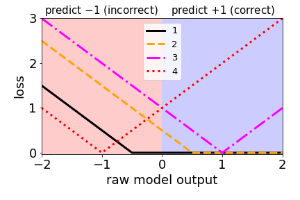
2.
This loss is very similar to the hinge loss used in SVMs (just shifted slightly).
#### Comparing the logistic and hinge losses
In this exercise you’ll create a plot of the logistic and hinge losses using their mathematical expressions, which are provided to you.
The loss function diagram from the video is shown below.
# Mathematical functions for logistic and hinge losses
def log_loss(raw_model_output):
   return np.log(1+np.exp(-raw_model_output))
def hinge_loss(raw_model_output):
   return np.maximum(0,1-raw_model_output)

# Create a grid of values and plot
grid = np.linspace(-2,2,1000)
plt.plot(grid, log_loss(grid), label='logistic')
plt.plot(grid, hinge_loss(grid), label='hinge')
plt.legend()
plt.show()

As you can see, these match up with the loss function diagrams above.
#### Implementing logistic regression
This is very similar to the earlier exercise where you implemented linear regression “from scratch” using
scipy.optimize.minimize
. However, this time we’ll minimize the logistic loss and compare with scikit-learn’s
LogisticRegression
(we’ve set
C
to a large value to disable regularization; more on this in Chapter 3!).
The
log_loss()
function from the previous exercise is already defined in your environment, and the
sklearn
breast cancer prediction dataset (first 10 features, standardized) is loaded into the variables
X
and
y
.
X.shape
(569, 10)


X[:2]
array([[ 1.09706398e+00, -2.07333501e+00,  1.26993369e+00,
         9.84374905e-01,  1.56846633e+00,  3.28351467e+00,
         2.65287398e+00,  2.53247522e+00,  2.21751501e+00,
         2.25574689e+00],
       [ 1.82982061e+00, -3.53632408e-01,  1.68595471e+00,
         1.90870825e+00, -8.26962447e-01, -4.87071673e-01,
        -2.38458552e-02,  5.48144156e-01,  1.39236330e-03,
        -8.68652457e-01]])


y[:2]
array([-1, -1])
# The logistic loss, summed over training examples
def my_loss(w):
    s = 0
    for i in range(y.shape[0]):
        raw_model_output = w@X[i]
        s = s + log_loss(raw_model_output * y[i])
    return s

# Returns the w that makes my_loss(w) smallest
w_fit = minimize(my_loss, X[0]).x
print(w_fit)

# Compare with scikit-learn's LogisticRegression
lr = LogisticRegression(fit_intercept=False, C=1000000).fit(X,y)
print(lr.coef_)
[ 1.03592182 -1.65378492  4.08331342 -9.40923002 -1.06786489  0.07892114
 -0.85110344 -2.44103305 -0.45285671  0.43353448]

[[ 1.03731085 -1.65339037  4.08143924 -9.40788356 -1.06757746  0.07895582
  -0.85072003 -2.44079089 -0.45271     0.43334997]]
minimize(my_loss, X[0])

      fun: 73.43533837769074
 hess_inv: array([[ 0.36738362, -0.00184266, -0.09662977, -0.38758529, -0.0212197 ,
        -0.05640658, -0.03033375,  0.21477573,  0.01029659, -0.03659313],
...
       [-0.03659313, -0.00862774,  0.09674119,  0.03706539,  0.02197145,
        -0.16126887,  0.06496472, -0.09572242,  0.01406182,  0.0907421 ]])
      jac: array([ 0.00000000e+00,  4.76837158e-06,  2.86102295e-06,  3.81469727e-06,
       -4.76837158e-06, -2.86102295e-06, -6.67572021e-06, -9.53674316e-07,
        9.53674316e-07, -7.62939453e-06])
  message: 'Optimization terminated successfully.'
     nfev: 660
      nit: 40
     njev: 55
   status: 0
  success: True
        x: array([ 1.03592182, -1.65378492,  4.08331342, -9.40923002, -1.06786489,
        0.07892114, -0.85110344, -2.44103305, -0.45285671,  0.43353448])
As you can see, logistic regression is just minimizing the loss function we’ve been looking at.
#### Regularized logistic regression
In Chapter 1, you used logistic regression on the handwritten digits data set. Here, we’ll explore the effect of L2 regularization.
The handwritten digits dataset is already loaded, split, and stored in the variables
X_train
,
y_train
,
X_valid
, and
y_valid
.
X_train[:2]
array([[ 0.,  0.,  7., 15., 15.,  5.,  0.,  0.,  0.,  6., 16., 12., 16.,
        12.,  0.,  0.,  0.,  1.,  7.,  0., 16., 10.,  0.,  0.,  0.,  0.,
         0., 10., 15.,  0.,  0.,  0.,  0.,  0.,  1., 16.,  7.,  0.,  0.,
         0.,  0.,  0., 10., 13.,  1.,  5.,  1.,  0.,  0.,  0., 12., 12.,
        13., 15.,  3.,  0.,  0.,  0., 10., 16., 13.,  3.,  0.,  0.],
       [ 0.,  0.,  0., 10., 11.,  0.,  0.,  0.,  0.,  0.,  3., 16., 10.,
         0.,  0.,  0.,  0.,  0.,  8., 16.,  0.,  0.,  0.,  0.,  0.,  0.,
        12., 14.,  0.,  0.,  0.,  0.,  0.,  0., 14., 16., 15.,  6.,  0.,
         0.,  0.,  0., 12., 16., 12., 15.,  6.,  0.,  0.,  0.,  7., 16.,
        10., 13., 14.,  0.,  0.,  0.,  0.,  9., 13., 11.,  6.,  0.]])

y_train[:2]
array([2, 6])
# Train and validaton errors initialized as empty list
train_errs = list()
valid_errs = list()

# Loop over values of C_value
for C_value in [0.001, 0.01, 0.1, 1, 10, 100, 1000]:
    # Create LogisticRegression object and fit
    lr = LogisticRegression(C=C_value)
    lr.fit(X_train, y_train)

    # Evaluate error rates and append to lists
    train_errs.append( 1.0 - lr.score(X_train, y_train) )
    valid_errs.append( 1.0 - lr.score(X_valid, y_valid) )

# Plot results
plt.semilogx(C_values, train_errs, C_values, valid_errs)
plt.legend(("train", "validation"))
plt.show()

As you can see, too much regularization (small
C
) doesn’t work well – due to underfitting – and too little regularization (large
C
) doesn’t work well either – due to overfitting.
#### Logistic regression and feature selection
In this exercise we’ll perform feature selection on the movie review sentiment data set using L1 regularization. The features and targets are already loaded for you in
X_train
and
y_train
.
We’ll search for the best value of
C
using scikit-learn’s
GridSearchCV()
.
# Specify L1 regularization
lr = LogisticRegression(penalty='l1')

# Instantiate the GridSearchCV object and run the search
searcher = GridSearchCV(lr, {'C':[0.001, 0.01, 0.1, 1, 10]})
searcher.fit(X_train, y_train)

# Report the best parameters
print("Best CV params", searcher.best_params_)

# Find the number of nonzero coefficients (selected features)
best_lr = searcher.best_estimator_
coefs = best_lr.coef_
print("Total number of features:", coefs.size)
print("Number of selected features:", np.count_nonzero(coefs))
Best CV params {'C': 1}
Total number of features: 2500
Number of selected features: 1220
#### Identifying the most positive and negative words
In this exercise we’ll try to interpret the coefficients of a logistic regression fit on the movie review sentiment dataset. The model object is already instantiated and fit for you in the variable
lr
.
In addition, the words corresponding to the different features are loaded into the variable
vocab
.
lr
LogisticRegression(C=1.0, class_weight=None, dual=False, fit_intercept=True,
          intercept_scaling=1, max_iter=100, multi_class='ovr', n_jobs=1,
          penalty='l2', random_state=None, solver='liblinear', tol=0.0001,
          verbose=0, warm_start=False)

vocab.shape
(2500,)

vocab[:3]
array(['the', 'and', 'a'], dtype='<U14')

vocab[-3:]
array(['birth', 'sorts', 'gritty'], dtype='<U14')
# Get the indices of the sorted cofficients
inds_ascending = np.argsort(lr.coef_.flatten())
inds_ascending
# array([1278,  427,  240, ..., 1458,  870,  493])

inds_descending = inds_ascending[::-1]
inds_descending
# array([ 493,  870, 1458, ...,  240,  427, 1278])


# Print the most positive words
print("Most positive words: ", end="")
for i in range(5):
    print(vocab[inds_descending][i], end=", ")
print("\n")

# Most positive words: favorite, superb, noir, knowing, loved,


# Print most negative words
print("Most negative words: ", end="")
for i in range(5):
    print(vocab[inds_ascending][i], end=", ")
print("\n")

# Most negative words: disappointing, waste, worst, boring, lame,


#### Regularization and probabilities
In this exercise, you will observe the effects of changing the regularization strength on the predicted probabilities.
A 2D binary classification dataset is already loaded into the environment as
X
and
y
.
X.shape
(20, 2)

X[:3]
array([[ 1.78862847,  0.43650985],
       [ 0.09649747, -1.8634927 ],
       [-0.2773882 , -0.35475898]])

y[:3]
array([-1, -1, -1])
# Set the regularization strength
model = LogisticRegression(C=1)

# Fit and plot
model.fit(X,y)
plot_classifier(X,y,model,proba=True)

# Predict probabilities on training points
prob = model.predict_proba(X)
print("Maximum predicted probability", np.max(prob))

C = 1
Maximum predicted probability 0.9761229966765974

C=0.1
Maximum predicted probability 0.8990965659596716
Smaller values of
C
lead to less confident predictions.
That’s because smaller
C
means more regularization, which in turn means smaller coefficients, which means raw model outputs closer to zero.
#### Visualizing easy and difficult examples
In this exercise, you’ll visualize the examples that the logistic regression model is most and least confident about by looking at the largest and smallest predicted probabilities.
The handwritten digits dataset is already loaded into the variables
X
and
y
. The
show_digit
function takes in an integer index and plots the corresponding image, with some extra information displayed above the image.
X.shape
(1797, 64)

X[0]
array([ 0.,  0.,  5., 13.,  9.,  1.,  0.,  0.,  0.,  0., 13., 15., 10.,
       15.,  5.,  0.,  0.,  3., 15.,  2.,  0., 11.,  8.,  0.,  0.,  4.,
       12.,  0.,  0.,  8.,  8.,  0.,  0.,  5.,  8.,  0.,  0.,  9.,  8.,
        0.,  0.,  4., 11.,  0.,  1., 12.,  7.,  0.,  0.,  2., 14.,  5.,
       10., 12.,  0.,  0.,  0.,  0.,  6., 13., 10.,  0.,  0.,  0.])

y[:3]
array([0, 1, 2])

show_digit?
Signature: show_digit(i, lr=None)
Docstring: <no docstring>
File:      /tmp/tmp12h5q4tk/<ipython-input-1-5d2049073a74>
Type:      function
lr = LogisticRegression()
lr.fit(X,y)

# Get predicted probabilities
proba = lr.predict_proba(X)

# Sort the example indices by their maximum probability
proba_inds = np.argsort(np.max(proba,axis=1))

# Show the most confident (least ambiguous) digit
show_digit(proba_inds[-1], lr)

# Show the least confident (most ambiguous) digit
show_digit(proba_inds[0], lr)


As you can see, the least confident example looks like a weird 4, and the most confident example looks like a very typical 0.


#### Counting the coefficients
If you fit a logistic regression model on a classification problem with 3 classes and 100 features, how many coefficients would you have, including intercepts?
303
100 coefficients + 1 intercept for each binary classifier. (A, B), (B, C), (C, A)
101 * 3 = 303
#### Fitting multi-class logistic regression
In this exercise, you’ll fit the two types of multi-class logistic regression, one-vs-rest and softmax/multinomial, on the handwritten digits data set and compare the results.
# Fit one-vs-rest logistic regression classifier
lr_ovr = LogisticRegression()
lr_ovr.fit(X_train, y_train)

print("OVR training accuracy:", lr_ovr.score(X_train, y_train))
print("OVR test accuracy    :", lr_ovr.score(X_test, y_test))

# Fit softmax classifier
lr_mn = LogisticRegression(multi_class='multinomial', solver='lbfgs')
lr_mn.fit(X_train, y_train)

print("Softmax training accuracy:", lr_mn.score(X_train, y_train))
print("Softmax test accuracy    :", lr_mn.score(X_test, y_test))
OVR training accuracy: 0.9948032665181886
OVR test accuracy    : 0.9644444444444444

Softmax training accuracy: 1.0
Softmax test accuracy    : 0.9688888888888889
As you can see, the accuracies of the two methods are fairly similar on this data set.
#### Visualizing multi-class logistic regression
In this exercise we’ll continue with the two types of multi-class logistic regression, but on a toy 2D data set specifically designed to break the one-vs-rest scheme.
The data set is loaded into
X_train
and
y_train
. The two logistic regression objects,
lr_mn
and
lr_ovr
, are already instantiated (with
C=100
), fit, and plotted.
Notice that
lr_ovr
never predicts the dark blue class… yikes! Let’s explore why this happens by plotting one of the binary classifiers that it’s using behind the scenes.


# Print training accuracies
print("Softmax     training accuracy:", lr_mn.score(X_train, y_train))
print("One-vs-rest training accuracy:", lr_ovr.score(X_train, y_train))

# Softmax     training accuracy: 0.996
# One-vs-rest training accuracy: 0.916

# Create the binary classifier (class 1 vs. rest)
lr_class_1 = LogisticRegression(C=100)
lr_class_1.fit(X_train, y_train==1)

# Plot the binary classifier (class 1 vs. rest)
plot_classifier(X_train, y_train==1, lr_class_1)

As you can see, the binary classifier incorrectly labels almost all points in class 1 (shown as red triangles in the final plot)! Thus, this classifier is not a very effective component of the one-vs-rest classifier.
In general, though, one-vs-rest often works well.
#### One-vs-rest SVM
As motivation for the next and final chapter on support vector machines, we’ll repeat the previous exercise with a non-linear SVM.
Instead of using
LinearSVC
, we’ll now use scikit-learn’s
SVC
object, which is a non-linear “kernel” SVM (much more on what this means in Chapter 4!). Again, your task is to create a plot of the binary classifier for class 1 vs. rest.
# We'll use SVC instead of LinearSVC from now on
from sklearn.svm import SVC

# Create/plot the binary classifier (class 1 vs. rest)
svm_class_1 = SVC()
svm_class_1.fit(X_train, y_train==1)
plot_classifier(X_train, y_train==1, svm_class_1)


The non-linear SVM works fine with one-vs-rest on this dataset because it learns to “surround” class 1.


#### Effect of removing examples
Support vectors are defined as training examples that influence the decision boundary. In this exercise, you’ll observe this behavior by removing non support vectors from the training set.
The wine quality dataset is already loaded into
X
and
y
(first two features only). (Note: we specify
lims
in
plot_classifier()
so that the two plots are forced to use the same axis limits and can be compared directly.)
X.shape
(178, 2)

X[:3]
array([[14.23,  1.71],
       [13.2 ,  1.78],
       [13.16,  2.36]])

set(y)
{0, 1, 2}
# Train a linear SVM
svm = SVC(kernel="linear")
svm.fit(X, y)
plot_classifier(X, y, svm, lims=(11,15,0,6))

# Make a new data set keeping only the support vectors
print("Number of original examples", len(X))
print("Number of support vectors", len(svm.support_))
X_small = X[svm.support_]
y_small = y[svm.support_]

# Train a new SVM using only the support vectors
svm_small = SVC(kernel="linear")
svm_small.fit(X_small, y_small)
plot_classifier(X_small, y_small, svm_small, lims=(11,15,0,6))


By the definition of support vectors, the decision boundaries of the two trained models are the same.


#### GridSearchCV warm-up
Increasing the RBF kernel hyperparameter
gamma
increases training accuracy.
In this exercise we’ll search for the
gamma
that maximizes cross-validation accuracy using scikit-learn’s
GridSearchCV
.
A binary version of the handwritten digits dataset, in which you’re just trying to predict whether or not an image is a “2”, is already loaded into the variables
X
and
y
.
set(y)
{False, True}

X.shape
(898, 64)

X[0]
array([ 0.,  1., 10., 15., 11.,  1.,  0.,  0.,  0.,  3.,  8.,  8., 11.,
       12.,  0.,  0.,  0.,  0.,  0.,  5., 14., 15.,  1.,  0.,  0.,  0.,
        0., 11., 15.,  2.,  0.,  0.,  0.,  0.,  0.,  4., 15.,  2.,  0.,
        0.,  0.,  0.,  0.,  0., 12., 10.,  0.,  0.,  0.,  0.,  3.,  4.,
       10., 16.,  1.,  0.,  0.,  0., 13., 16., 15., 10.,  0.,  0.])
# Instantiate an RBF SVM
svm = SVC()

# Instantiate the GridSearchCV object and run the search
parameters = {'gamma':[0.00001, 0.0001, 0.001, 0.01, 0.1]}
searcher = GridSearchCV(svm, param_grid=parameters)
searcher.fit(X, y)

# Report the best parameters
print("Best CV params", searcher.best_params_)

# Best CV params {'gamma': 0.001}
Larger values of
gamma
are better for training accuracy, but cross-validation helped us find something different (and better!).
#### Jointly tuning gamma and C with GridSearchCV
In the previous exercise the best value of
gamma
was 0.001 using the default value of
C
, which is 1. In this exercise you’ll search for the best combination of
C
and
gamma
using
GridSearchCV
.
As in the previous exercise, the 2-vs-not-2 digits dataset is already loaded, but this time it’s split into the variables
X_train
,
y_train
,
X_test
, and
y_test
.
Even though cross-validation already splits the training set into parts, it’s often a good idea to hold out a separate test set to make sure the cross-validation results are sensible.
# Instantiate an RBF SVM
svm = SVC()

# Instantiate the GridSearchCV object and run the search
parameters = {'C':[0.1, 1, 10], 'gamma':[0.00001, 0.0001, 0.001, 0.01, 0.1]}
searcher = GridSearchCV(svm, param_grid=parameters)
searcher.fit(X_train, y_train)

# Report the best parameters and the corresponding score
print("Best CV params", searcher.best_params_)
print("Best CV accuracy", searcher.best_score_)

# Report the test accuracy using these best parameters
print("Test accuracy of best grid search hypers:", searcher.score(X_test, y_test))
Best CV params {'C': 10, 'gamma': 0.0001}
Best CV accuracy 0.9988864142538976
Test accuracy of best grid search hypers: 0.9988876529477196
Note that the best value of
gamma
, 0.0001, is different from the value of 0.001 that we got in the previous exercise, when we fixed
C=1
. Hyperparameters can affect each other!


#### An advantage of SVMs
Having a limited number of support vectors makes kernel SVMs computationally efficient.
#### An advantage of logistic regression
It naturally outputs meaningful probabilities.
#### Using SGDClassifier
In this final coding exercise, you’ll do a hyperparameter search over the regularization type, regularization strength, and the loss (logistic regression vs. linear SVM) using
SGDClassifier()
.
X_train.shape
(1257, 64)

X_train[0]
array([ 0.,  0.,  2., 10., 16., 11.,  1.,  0.,  0.,  0., 13., 13., 10.,
       16.,  8.,  0.,  0.,  4., 14.,  1.,  8., 14.,  1.,  0.,  0.,  4.,
       15., 12., 15.,  8.,  0.,  0.,  0.,  0.,  6.,  7., 14.,  5.,  0.,
        0.,  0.,  1.,  2.,  0., 12.,  5.,  0.,  0.,  0.,  8., 15.,  6.,
       13.,  4.,  0.,  0.,  0.,  0.,  5., 11., 16.,  3.,  0.,  0.])

set(y_train)
{0, 1, 2, 3, 4, 5, 6, 7, 8, 9}
# We set random_state=0 for reproducibility
linear_classifier = SGDClassifier(random_state=0)

# Instantiate the GridSearchCV object and run the search
parameters = {'alpha':[0.00001, 0.0001, 0.001, 0.01, 0.1, 1],
             'loss':['hinge', 'log'], 'penalty':['l1', 'l2']}
searcher = GridSearchCV(linear_classifier, parameters, cv=10)
searcher.fit(X_train, y_train)

# Report the best parameters and the corresponding score
print("Best CV params", searcher.best_params_)
print("Best CV accuracy", searcher.best_score_)
print("Test accuracy of best grid search hypers:", searcher.score(X_test, y_test))
Best CV params {'alpha': 0.0001, 'loss': 'hinge', 'penalty': 'l1'}
Best CV accuracy 0.94351630867144
Test accuracy of best grid search hypers: 0.9592592592592593
One advantage of
SGDClassifier
is that it’s very fast – this would have taken a lot longer with
LogisticRegression
or
LinearSVC
.
The End.
Thank you for reading.