Introduction to TensorFlow in Python

This is the memo of the 14th course (23 courses in all) of ‘Machine Learning Scientist with Python’ skill track.

You can find the original course HERE .

### Course Description

Not long ago, cutting-edge computer vision algorithms couldn’t differentiate between images of cats and dogs. Today, a skilled data scientist equipped with nothing more than a laptop can classify tens of thousands of objects with greater accuracy than the human eye. In this course, you will use TensorFlow 2.0 to develop, train, and make predictions with the models that have powered major advances in recommendation systems, image classification, and FinTech. You will learn both high-level APIs, which will enable you to design and train deep learning models in 15 lines of code, and low-level APIs, which will allow you to move beyond off-the-shelf routines. You will also learn to accurately predict housing prices, credit card borrower defaults, and images of sign language gestures.

### Table of contents

• Introduction to TensorFlow
• Linear models
• Neural Networks
• High Level APIs

1. Introduction to TensorFlow

1.1 Constants and variables

1.1.1 Defining data as constants

Throughout this course, we will use tensorflow version 2.0 and will exclusively import the submodules needed to complete each exercise. This will usually be done for you, but you will do it in this exercise by importing constant from tensorflow .

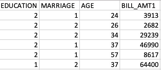
After you have imported constant , you will use it to transform a numpy array, credit_numpy , into a tensorflow constant, credit_constant . This array contains feature columns from a dataset on credit card holders and is previewed in the image below. We will return to this dataset in later chapters.

Note that tensorflow version 2.0 allows you to use data as either a numpy array or a tensorflow constant object. Using a constant will ensure that any operations performed with that object are done in tensorflow .

# Import constant from TensorFlow
from tensorflow import constant

# Convert the credit_numpy array into a tensorflow constant
credit_constant = constant(credit_numpy)

# Print constant datatype
print('The datatype is:', credit_constant.dtype)

# Print constant shape
print('The shape is:', credit_constant.shape)

The datatype is: <dtype: 'float64'>
The shape is: (30000, 4)

credit_numpy
array([[ 2.0000e+00,  1.0000e+00,  2.4000e+01,  3.9130e+03],
       [ 2.0000e+00,  2.0000e+00,  2.6000e+01,  2.6820e+03],
       [ 2.0000e+00,  2.0000e+00,  3.4000e+01,  2.9239e+04],
       ...,
       [ 2.0000e+00,  2.0000e+00,  3.7000e+01,  3.5650e+03],
       [ 3.0000e+00,  1.0000e+00,  4.1000e+01, -1.6450e+03],
       [ 2.0000e+00,  1.0000e+00,  4.6000e+01,  4.7929e+04]])

credit_constant
<tf.Tensor: id=0, shape=(30000, 4), dtype=float64, numpy=
array([[ 2.0000e+00,  1.0000e+00,  2.4000e+01,  3.9130e+03],
       [ 2.0000e+00,  2.0000e+00,  2.6000e+01,  2.6820e+03],
       [ 2.0000e+00,  2.0000e+00,  3.4000e+01,  2.9239e+04],
       ...,
       [ 2.0000e+00,  2.0000e+00,  3.7000e+01,  3.5650e+03],
       [ 3.0000e+00,  1.0000e+00,  4.1000e+01, -1.6450e+03],
       [ 2.0000e+00,  1.0000e+00,  4.6000e+01,  4.7929e+04]])>

Excellent! You now understand how constants are used in tensorflow . In the following exercise, you’ll practice defining variables.

1.1.2 Defining variables

Unlike a constant, a variable’s value can be modified. This will be quite useful when we want to train a model by updating its parameters. Constants can’t be used for this purpose, so variables are the natural choice.

Let’s try defining and working with a variable. Note that Variable() , which is used to create a variable tensor, has been imported from tensorflow and is available to use in the exercise.

from tensorflow import Variable

# Define the 1-dimensional variable A1
A1 = Variable([1, 2, 3, 4])

# Print the variable A1
print(A1)

# Convert A1 to a numpy array and assign it to B1
B1 = A1.numpy()

# Print B1
print(B1)

<tf.Variable 'Variable:0' shape=(4,) dtype=int32, numpy=array([1, 2, 3, 4], dtype=int32)>
[1 2 3 4]

Nice work! In our next exercise, we’ll review how to check the properties of a tensor after it is already defined.

1.2 Basic operations

1.2.1 Performing element-wise multiplication

Element-wise multiplication in TensorFlow is performed using two tensors with identical shapes. This is because the operation multiplies elements in corresponding positions in the two tensors. An example of an element-wise multiplication, denoted by the ⊙ symbol, is shown below:

In this exercise, you will perform element-wise multiplication, paying careful attention to the shape of the tensors you multiply. Note that multiply() , constant() , and ones_like() have been imported for you.

# Define tensors A1 and A23 as constants
A1 = constant([1, 2, 3, 4])
A23 = constant([[1, 2, 3], [1, 6, 4]])

# Define B1 and B23 to have the correct shape
B1 = ones_like(A1)
B23 = ones_like(A23)

# Perform element-wise multiplication
C1 = multiply(A1,B1)
C23 = multiply(A23,B23)

# Print the tensors C1 and C23
print('C1: {}'.format(C1.numpy()))
print('C23: {}'.format(C23.numpy()))

C1: [1 2 3 4]
C23: [[1 2 3]
 [1 6 4]]

ones_like(A1)
<tf.Tensor: id=12, shape=(4,), dtype=int32, numpy=array([1, 1, 1, 1], dtype=int32)>


ones_like(A23)
<tf.Tensor: id=15, shape=(2, 3), dtype=int32, numpy=
array([[1, 1, 1],
       [1, 1, 1]], dtype=int32)>

Excellent work! Notice how performing element-wise multiplication with tensors of ones leaves the original tensors unchanged.

1.2.2 Making predictions with matrix multiplication

In later chapters, you will learn to train linear regression models. This process will yield a vector of parameters that can be multiplied by the input data to generate predictions. In this exercise, you will use input data, features , and a target vector, bill , which are taken from a credit card dataset we will use later in the course.

The matrix of input data, features , contains two columns: education level and age. The target vector, bill , is the size of the credit card borrower’s bill.

Since we have not trained the model, you will enter a guess for the values of the parameter vector, params . You will then use matmul() to perform matrix multiplication of features by params to generate predictions, billpred , which you will compare with bill . Note that we have imported matmul() and constant() .

# Define features, params, and bill as constants
features = constant([[2, 24], [2, 26], [2, 57], [1, 37]])
params = constant([[1000], [150]])
bill = constant([[3913], [2682], [8617], [64400]])

# Compute billpred using features and params
billpred = matmul(features,params)

# Compute and print the error
error = bill - billpred
print(error.numpy())

[[-1687]
 [-3218]
 [-1933]
 [57850]]

billpred
<tf.Tensor: id=15, shape=(4, 1), dtype=int32, numpy=
array([[ 5600],
       [ 5900],
       [10550],
       [ 6550]], dtype=int32)>

Nice job! Understanding matrix multiplication will make things simpler when we start making predictions with linear models.

1.2.3 Summing over tensor dimensions

You’ve been given a matrix, wealth . This contains the value of bond and stock wealth for five individuals in thousands of dollars.

The first column corresponds to bonds and the second corresponds to stocks. Each row gives the bond and stock wealth for a single individual. Use wealth , reduce_sum() , and .numpy() to determine which statements are correct about wealth .

reduce_sum(wealth,0).numpy()
# array([ 50, 122], dtype=int32)

reduce_sum(wealth,1).numpy()
# array([61,  9, 64,  3, 35], dtype=int32)

reduce_sum(wealth).numpy()
# 172

Combined, the 5 individuals hold $50,000 in bonds.

Excellent work! Understanding how to sum over tensor dimensions will be helpful when preparing datasets and training models.

1.3 Advanced operations

1.3.1 Reshaping tensors

Later in the course, you will classify images of sign language letters using a neural network. In some cases, the network will take 1-dimensional tensors as inputs, but your data will come in the form of images, which will either be either 2- or 3-dimensional tensors, depending on whether they are grayscale or color images.

The figure below shows grayscale and color images of the sign language letter A. The two images have been imported for you and converted to the numpy arrays gray_tensor and color_tensor . Reshape these arrays into 1-dimensional vectors using the reshape operation, which has been imported for you from tensorflow . Note that the shape of gray_tensor is 28×28 and the shape of color_tensor is 28x28x3.

# Reshape the grayscale image tensor into a vector
gray_vector = reshape(gray_tensor, (28*28, 1))

# Reshape the color image tensor into a vector
color_vector = reshape(color_tensor, (28*28*3, 1))

Excellent work! Notice that there are 3 times as many elements in color_vector as there are in gray_vector , since color_tensor has 3 color channels.

1.3.2 Optimizing with gradients

You are given a loss function, y=x2y=x2, which you want to minimize. You can do this by computing the slope using the GradientTape() operation at different values of x . If the slope is positive, you can decrease the loss by lowering x . If it is negative, you can decrease it by increasing x . This is how gradient descent works.

In practice, you will use a high level tensorflow operation to perform gradient descent automatically. In this exercise, however, you will compute the slope at x values of -1, 1, and 0. The following operations are available: GradientTape() , multiply() , and Variable() .

def compute_gradient(x0):
  	# Define x as a variable with an initial value of x0
	x = Variable(x0)
	with GradientTape() as tape:
		tape.watch(x)
        # Define y using the multiply operation
		y = multiply(x,x)
    # Return the gradient of y with respect to x
	return tape.gradient(y, x).numpy()

# Compute and print gradients at x = -1, 1, and 0
print(compute_gradient(-1.0))
# -2.0
print(compute_gradient(1.0))
# 2.0
print(compute_gradient(0.0))
# 0.0

Excellent work! Notice that the slope is positive at x = 1, which means that we can lower the loss by reducing x . The slope is negative at x = -1, which means that we can lower the loss by increasing x . The slope at x = 0 is 0, which means that we cannot lower the loss by either increasing or decreasing x . This is because the loss is minimized at x = 0.

1.3.3 Working with image data

You are given a black-and-white image of a letter, which has been encoded as a tensor, letter . You want to determine whether the letter is an X or a K. You don’t have a trained neural network, but you do have a simple model, model , which can be used to classify letter .

The 3×3 tensor, letter , and the 1×3 tensor, model , are available in the Python shell. You can determine whether letter is a K by multiplying letter by model , summing over the result, and then checking if it is equal to 1. As with more complicated models, such as neural networks, model is a collection of weights, arranged in a tensor.

Note that the functions reshape() , matmul() , and reduce_sum() have been imported from tensorflow and are available for use.

letter
array([[1., 0., 1.],
       [1., 1., 0.],
       [1., 0., 1.]], dtype=float32)

# Reshape model from a 1x3 to a 3x1 tensor
model = reshape(model, (3, 1))

# Multiply letter by model
output = matmul(letter, model)

# Sum over output and print prediction using the numpy method
prediction = reduce_sum(output)
print(prediction.numpy())
# 1.0

Excellent work! Your model found that prediction =1.0 and correctly classified the letter as a K. In the coming chapters, you will use data to train a model, model , and then combine this with matrix multiplication, matmul(letter, model) , as we have done here, to make predictions about the classes of objects.

2. Linear models

2.1 Input data

2.1.1 Load data using pandas

Before you can train a machine learning model, you must first import data. There are several valid ways to do this, but for now, we will use a simple one-liner from pandas : pd.read_csv() . Recall from the video that the first argument specifies the path or URL. All other arguments are optional.

In this exercise, you will import the King County housing dataset, which we will use to train a linear model later in the chapter.

# Import pandas under the alias pd
import pandas as pd

# Assign the path to a string variable named data_path
data_path = 'kc_house_data.csv'

# Load the dataset as a dataframe named housing
housing = pd.read_csv(data_path)

# Print the price column of housing
print(housing['price'])

Excellent work! Notice that you did not have to specify a delimiter with the sep parameter, since the dataset was stored in the default, comma-separated format.

2.1.2 Setting the data type

In this exercise, you will both load data and set its type. Note that housing is available and pandas has been imported as pd . You will import numpy and tensorflow , and define tensors that are usable in tensorflow using columns in housing with a given data type. Recall that you can select the price column, for instance, from housing using housing['price'] .

# Import numpy and tensorflow with their standard aliases
import numpy as np
import tensorflow as tf

# Use a numpy array to define price as a 32-bit float
price = np.array(housing['price'], np.float)

# Define waterfront as a Boolean using cast
waterfront = tf.cast(housing['waterfront'], tf.bool)

# Print price and waterfront
print(price)
print(waterfront)

[221900. 538000. 180000. ... 402101. 400000. 325000.]
tf.Tensor([False False False ... False False False], shape=(21613,), dtype=bool)

Great job! Notice that printing price yielded a numpy array; whereas printing waterfront yielded a tf.Tensor() .

2.2 Loss functions

2.2.1 Loss functions in TensorFlow

In this exercise, you will compute the loss using data from the King County housing dataset. You are given a target, price , which is a tensor of house prices, and predictions , which is a tensor of predicted house prices. You will evaluate the loss function and print out the value of the loss.

# Import the keras module from tensorflow
from tensorflow import keras

# Compute the mean squared error (mse)
loss = keras.losses.mse(price, predictions)

# Print the mean squared error (mse)
print(loss.numpy())
# 141171604777.12717


# Compute the mean absolute error (mae)
loss = keras.losses.mae(price, predictions)

# Print the mean absolute error (mae)
print(loss.numpy())
# 268827.99302087986

Great work! You may have noticed that the MAE was much smaller than the MSE, even though price and predictions were the same. This is because the different loss functions penalize deviations of predictions from price differently. MSE does not like large deviations and punishes them harshly.

2.2.2 Modifying the loss function

In the previous exercise, you defined a tensorflow loss function and then evaluated it once for a set of actual and predicted values. In this exercise, you will compute the loss within another function called loss_function() , which first generates predicted values from the data and variables. The purpose of this is to construct a function of the trainable model variables that returns the loss. You can then repeatedly evaluate this function for different variable values until you find the minimum. In practice, you will pass this function to an optimizer in tensorflow . Note that features and targets have been defined and are available. Additionally, Variable , float32 , and keras are available.

import tensorflow as tf
from tensorflow import Variable
from tensorflow import keras

# Initialize a variable named scalar
scalar = Variable(1.0, tf.float32)

# Define the model
def model(scalar, features = features):
  	return scalar * features

# Define a loss function
def loss_function(scalar, features = features, targets = targets):
	# Compute the predicted values
	predictions = model(scalar, features)

	# Return the mean absolute error loss
	return keras.losses.mae(targets, predictions)

# Evaluate the loss function and print the loss
print(loss_function(scalar).numpy())
# 3.0

Great work! As you will see in the following lessons, this exercise was the equivalent of evaluating the loss function for a linear regression where the intercept is 0.

2.3 Linear regression

2.3.1 Set up a linear regression

A univariate linear regression identifies the relationship between a single feature and the target tensor. In this exercise, we will use a property’s lot size and price. Just as we discussed in the video, we will take the natural logarithms of both tensors, which are available as price_log and size_log .

In this exercise, you will define the model and the loss function. You will then evaluate the loss function for two different values of intercept and slope . Remember that the predicted values are given by intercept + features*slope . Additionally, note that keras.losses.mse() is available for you. Furthermore, slope and intercept have been defined as variables.

# Define a linear regression model
def linear_regression(intercept, slope, features = size_log):
	return intercept + slope*features

# Set loss_function() to take the variables as arguments
def loss_function(intercept, slope, features = size_log, targets = price_log):
	# Set the predicted values
	predictions = linear_regression(intercept, slope, features)

    # Return the mean squared error loss
	return keras.losses.mse(targets, predictions)

# Compute the loss for different slope and intercept values
print(loss_function(0.1, 0.1).numpy())
print(loss_function(0.1, 0.5).numpy())
# 145.44652
# 71.866

Great work! In the next exercise, you will actually run the regression and train intercept and slope .

2.3.2 Train a linear model

In this exercise, we will pick up where the previous exercise ended. The intercept and slope, intercept and slope , have been defined and initialized. Additionally, a function has been defined, loss_function(intercept, slope) , which computes the loss using the data and model variables.

You will now define an optimization operation as opt . You will then train a univariate linear model by minimizing the loss to find the optimal values of intercept and slope . Note that the opt operation will try to move closer to the optimum with each step, but will require many steps to find it. Thus, you must repeatedly execute the operation.

# Initialize an adam optimizer
opt = keras.optimizers.Adam(0.5)

for j in range(100):
	# Apply minimize, pass the loss function, and supply the variables
	opt.minimize(lambda: loss_function(intercept, slope), var_list=[intercept, slope])

	# Print every 10th value of the loss
	if j % 10 == 0:
		print(loss_function(intercept, slope).numpy())

# Plot data and regression line
plot_results(intercept, slope)

9.669481
11.726705
1.1193314
1.6605749
0.7982892
0.8017315
0.6106562
0.59997994
0.5811015
0.5576157

Excellent! Notice that we printed loss_function(intercept, slope) every 10th execution for 100 executions. Each time, the loss got closer to the minimum as the optimizer moved the slope and intercept parameters closer to their optimal values.

2.3.3 Multiple linear regression

In most cases, performing a univariate linear regression will not yield a model that is useful for making accurate predictions. In this exercise, you will perform a multiple regression, which uses more than one feature.

You will use price_log as your target and size_log and bedrooms as your features. Each of these tensors has been defined and is available. You will also switch from using the the mean squared error loss to the mean absolute error loss: keras.losses.mae() . Finally, the predicted values are computed as follows: params[0] + feature1*params[1] + feature2*params[2] . Note that we’ve defined a vector of parameters, params , as a variable, rather than using three variables. Here, params[0] is the intercept and params[1] and params[2] are the slopes.

# Define the linear regression model
def linear_regression(params, feature1 = size_log, feature2 = bedrooms):
	return params[0] + feature1*params[1] + feature2*params[2]

# Define the loss function
def loss_function(params, targets = price_log, feature1 = size_log, feature2 = bedrooms):
	# Set the predicted values
	predictions = linear_regression(params, feature1, feature2)

	# Use the mean absolute error loss
	return keras.losses.mae(targets, predictions)

# Define the optimize operation
opt = keras.optimizers.Adam()

# Perform minimization and print trainable variables
for j in range(10):
	opt.minimize(lambda: loss_function(params), var_list=[params])
	print_results(params)

loss: 12.418, intercept: 0.101, slope_1: 0.051, slope_2: 0.021
loss: 12.404, intercept: 0.102, slope_1: 0.052, slope_2: 0.022
loss: 12.391, intercept: 0.103, slope_1: 0.053, slope_2: 0.023
loss: 12.377, intercept: 0.104, slope_1: 0.054, slope_2: 0.024
loss: 12.364, intercept: 0.105, slope_1: 0.055, slope_2: 0.025
loss: 12.351, intercept: 0.106, slope_1: 0.056, slope_2: 0.026
loss: 12.337, intercept: 0.107, slope_1: 0.057, slope_2: 0.027
loss: 12.324, intercept: 0.108, slope_1: 0.058, slope_2: 0.028
loss: 12.311, intercept: 0.109, slope_1: 0.059, slope_2: 0.029
loss: 12.297, intercept: 0.110, slope_1: 0.060, slope_2: 0.030

Great job! Note that params[2] tells us how much the price will increase in percentage terms if we add one more bedroom. You could train params[2] and the other model parameters by increasing the number of times we iterate over opt .

2.4 Batch training

2.4.1 Preparing to batch train

Before we can train a linear model in batches, we must first define variables, a loss function, and an optimization operation. In this exercise, we will prepare to train a model that will predict price_batch , a batch of house prices, using size_batch , a batch of lot sizes in square feet. In contrast to the previous lesson, we will do this by loading batches of data using pandas , converting it to numpy arrays, and then using it to minimize the loss function in steps.

Variable() , keras() , and float32 have been imported for you. Note that you should not set default argument values for either the model or loss function, since we will generate the data in batches during the training process.

# Define the intercept and slope
intercept = Variable(10.0, float32)
slope = Variable(0.5, float32)

# Define the model
def linear_regression(intercept, slope, features):
	# Define the predicted values
	return intercept + slope*features

# Define the loss function
def loss_function(intercept, slope, targets, features):
	# Define the predicted values
	predictions = linear_regression(intercept, slope, features)

 	# Define the MSE loss
	return keras.losses.mse(targets, predictions)

Excellent work! Notice that we did not use default argument values for the input data, features and targets . This is because the input data has not been defined in advance. Instead, with batch training, we will load it during the training process.

2.4.2 Training a linear model in batches

In this exercise, we will train a linear regression model in batches, starting where we left off in the previous exercise. We will do this by stepping through the dataset in batches and updating the model’s variables, intercept and slope , after each step. This approach will allow us to train with datasets that are otherwise too large to hold in memory.

Note that the loss function, loss_function(intercept, slope, targets, features) , has been defined for you. Additionally, keras has been imported for you and numpy is available as np . The trainable variables should be entered into var_list in the order in which they appear as loss function arguments.

# Initialize adam optimizer
opt = keras.optimizers.Adam()

# Load data in batches
for batch in pd.read_csv('kc_house_data.csv', chunksize=100):
	size_batch = np.array(batch['sqft_lot'], np.float32)

	# Extract the price values for the current batch
	price_batch = np.array(batch['price'], np.float32)

	# Complete the loss, fill in the variable list, and minimize
	opt.minimize(lambda: loss_function(intercept, slope, price_batch, size_batch), var_list=[intercept, slope])

# Print trained parameters
print(intercept.numpy(), slope.numpy())
# 10.217888 0.7016

Great work! Batch training will be very useful when you train neural networks, which we will do next.

3. Neural Networks

3.1 Dense layers

3.1.1 The linear algebra of dense layers

There are two ways to define a dense layer in tensorflow . The first involves the use of low-level, linear algebraic operations. The second makes use of high-level keras operations. In this exercise, we will use the first method to construct the network shown in the image below.

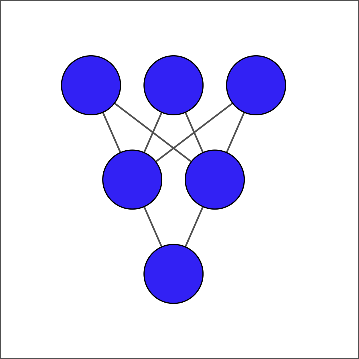
The input layer contains 3 features — education, marital status, and age — which are available as borrower_features . The hidden layer contains 2 nodes and the output layer contains a single node.

For each layer, you will take the previous layer as an input, initialize a set of weights, compute the product of the inputs and weights, and then apply an activation function. Note that Variable() , ones() , matmul() , and keras() have been imported from tensorflow .

# Initialize bias1
bias1 = Variable(1.0)

# Initialize weights1 as 3x2 variable of ones
weights1 = Variable(ones((3, 2)))

# Perform matrix multiplication of borrower_features and weights1
product1 = matmul(borrower_features,weights1)

# Apply sigmoid activation function to product1 + bias1
dense1 = keras.activations.sigmoid(product1 + bias1)

# Print shape of dense1
print("\n dense1's output shape: {}".format(dense1.shape))
# dense1's output shape: (1, 2)

# From previous step
bias1 = Variable(1.0)
weights1 = Variable(ones((3, 2)))
product1 = matmul(borrower_features, weights1)
dense1 = keras.activations.sigmoid(product1 + bias1)

# Initialize bias2 and weights2
bias2 = Variable(1.0)
weights2 = Variable(ones((2, 1)))

# Perform matrix multiplication of dense1 and weights2
product2 = matmul(dense1, weights2)

# Apply activation to product2 + bias2 and print the prediction
prediction = keras.activations.sigmoid(product2 + bias2)
print('\n prediction: {}'.format(prediction.numpy()[0,0]))
print('\n actual: 1')

 prediction: 0.9525741338729858

 actual: 1

Excellent work! Our model produces predicted values in the interval between 0 and 1. For the example we considered, the actual value was 1 and the predicted value was a probability between 0 and 1. This, of course, is not meaningful, since we have not yet trained our model’s parameters.

3.1.2 The low-level approach with multiple examples

In this exercise, we’ll build further intuition for the low-level approach by constructing the first dense hidden layer for the case where we have multiple examples. We’ll assume the model is trained and the first layer weights, weights1 , and bias, bias1 , are available. We’ll then perform matrix multiplication of the borrower_features tensor by the weights1 variable. Recall that the borrower_features tensor includes education, marital status, and age. Finally, we’ll apply the sigmoid function to the elements of products1 + bias1 , yielding dense1 .

Note that matmul() and keras() have been imported from tensorflow .

# Compute the product of borrower_features and weights1
products1 = matmul(borrower_features,weights1)

# Apply a sigmoid activation function to products1 + bias1
dense1 = keras.activations.sigmoid(products1+bias1)

# Print the shapes of borrower_features, weights1, bias1, and dense1
print('\n shape of borrower_features: ', borrower_features.shape)
#  shape of borrower_features:  (5, 3)

print('\n shape of weights1: ', weights1.shape)
#  shape of weights1:  (3, 2)

print('\n shape of bias1: ', bias1.shape)
#  shape of bias1:  (1,)

print('\n shape of dense1: ', dense1.shape)
#  shape of dense1:  (5, 2)

Good job! Note that our input data, borrower_features , is 5×3 because it consists of 5 examples for 3 features. The shape of weights1 is 3×2, as it was in the previous exercise, since it does not depend on the number of examples. Additionally, bias1 is a scalar. Finally, dense1 is 5×2, which means that we can multiply it by the following set of weights, weights2 , which we defined to be 2×1 in the previous exercise.

3.1.3 Using the dense layer operation

We’ve now seen how to define dense layers in tensorflow using linear algebra. In this exercise, we’ll skip the linear algebra and let keras work out the details. This will allow us to construct the network below, which has 2 hidden layers and 10 features, using less code than we needed for the network with 1 hidden layer and 3 features.

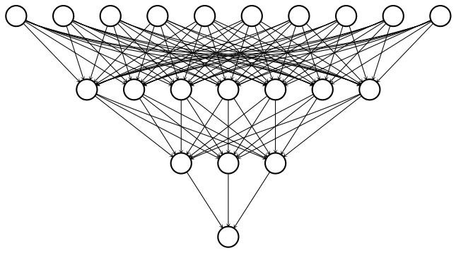
To construct this network, we’ll need to define three dense layers, each of which takes the previous layer as an input, multiplies it by weights, and applies an activation function. Note that input data has been defined and is available as a 100×10 tensor: borrower_features . Additionally, the keras.layers module is available.

# Define the first dense layer
dense1 = keras.layers.Dense(7, activation='sigmoid')(borrower_features)

# Define a dense layer with 3 output nodes
dense2 = keras.layers.Dense(3, activation='sigmoid')(dense1)

# Define a dense layer with 1 output node
predictions = keras.layers.Dense(1, activation='sigmoid')(dense2)

# Print the shapes of dense1, dense2, and predictions
print('\n shape of dense1: ', dense1.shape)
#  shape of dense1:  (100, 7)

print('\n shape of dense2: ', dense2.shape)
#  shape of dense2:  (100, 3)

print('\n shape of predictions: ', predictions.shape)
#  shape of predictions:  (100, 1)

Great work! With just 8 lines of code, you were able to define 2 dense hidden layers and an output layer. This is the advantage of using high-level operations in tensorflow . Note that each layer has 100 rows because the input data contains 100 examples.

3.2 Activation functions

3.2.1 Binary classification problems

In this exercise, you will again make use of credit card data. The target variable, default , indicates whether a credit card holder defaults on her payment in the following period. Since there are only two options–default or not–this is a binary classification problem. While the dataset has many features, you will focus on just three: the size of the three latest credit card bills. Finally, you will compute predictions from your untrained network, outputs , and compare those the target variable, default .

The tensor of features has been loaded and is available as bill_amounts . Additionally, the constant() , float32 , and keras.layers.Dense() operations are available.

# Construct input layer from features
inputs = constant(bill_amounts)

# Define first dense layer
dense1 = keras.layers.Dense(3, activation='relu')(inputs)

# Define second dense layer
dense2 = keras.layers.Dense(2, activation='relu')(dense1)

# Define output layer
outputs = keras.layers.Dense(1, activation='sigmoid')(dense2)

# Print error for first five examples
error = default[:5] - outputs.numpy()[:5]
print(error)

    [[ 0.0000000e+00]
     [ 3.4570694e-05]
     [-1.0000000e+00]
     [-1.0000000e+00]
     [-1.0000000e+00]]

Excellent work! If you run the code several times, you’ll notice that the errors change each time. This is because you’re using an untrained model with randomly initialized parameters. Furthermore, the errors fall on the interval between -1 and 1 because default is a binary variable that takes on values of 0 and 1 and outputs is a probability between 0 and 1.

3.2.2 Multiclass classification problems

In this exercise, we expand beyond binary classification to cover multiclass problems. A multiclass problem has targets that can take on three or more values. In the credit card dataset, the education variable can take on 6 different values, each corresponding to a different level of education. We will use that as our target in this exercise and will also expand the feature set from 3 to 10 columns.

As in the previous problem, you will define an input layer, dense layers, and an output layer. You will also print the untrained model’s predictions, which are probabilities assigned to the classes. The tensor of features has been loaded and is available as borrower_features . Additionally, the constant() , float32 , and keras.layers.Dense() operations are available.

import tensorflow as tf
# Construct input layer from borrower features
inputs = constant(borrower_features,tf.float32)

# Define first dense layer
dense1 = keras.layers.Dense(10, activation='sigmoid')(inputs)

# Define second dense layer
dense2 = keras.layers.Dense(8, activation='relu')(dense1)

# Define output layer
outputs = keras.layers.Dense(6, activation='softmax')(dense2)

# Print first five predictions
print(outputs.numpy()[:5])

    [[0.17133032 0.16293828 0.14702542 0.17789574 0.16075517 0.18005505]
     [0.15597914 0.17065835 0.1275746  0.2044413  0.16524555 0.17610106]
     [0.15597914 0.17065835 0.1275746  0.2044413  0.16524555 0.17610106]
     [0.17133032 0.16293828 0.14702542 0.17789574 0.16075517 0.18005505]
     [0.07605464 0.17264706 0.15399623 0.2247733  0.1516134  0.22091544]]

Great work! Notice that each row of outputs sums to one. This is because a row contains the predicted class probabilities for one example. As with the previous exercise, our predictions are not yet informative, since we are using an untrained model with randomly initialized parameters. This is why the model tends to assign similar probabilities to each class.

3.3 Optimizers

3.3.1 The dangers of local minima

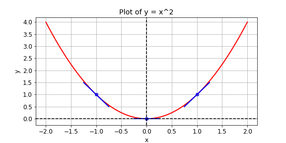
Consider the plot of the following loss function, loss_function() , which contains a global minimum, marked by the dot on the right, and several local minima, including the one marked by the dot on the left.

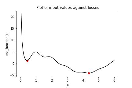
In this exercise, you will try to find the global minimum of loss_function() using keras.optimizers.SGD() . You will do this twice, each time with a different initial value of the input to loss_function() . First, you will use x_1 , which is a variable with an initial value of 6.0. Second, you will use x_2 , which is a variable with an initial value of 0.3. Note that loss_function() has been defined and is available.

# Initialize x_1 and x_2
x_1 = Variable(6.0,float32)
x_2 = Variable(0.3,float32)

# Define the optimization operation
opt = keras.optimizers.SGD(learning_rate=0.01)

for j in range(100):
	# Perform minimization using the loss function and x_1
	opt.minimize(lambda: loss_function(x_1), var_list=[x_1])
	# Perform minimization using the loss function and x_2
	opt.minimize(lambda: loss_function(x_2), var_list=[x_2])

# Print x_1 and x_2 as numpy arrays
print(x_1.numpy(), x_2.numpy())
# 4.3801394 0.42052683

Great work! Notice that we used the same optimizer and loss function, but two different initial values. When we started at 6.0 with x_1 , we found the global minimum at 4.38, marked by the dot on the right. When we started at 0.3, we stopped around 0.42 with x_2 , the local minimum marked by a dot on the far left.

3.3.2 Avoiding local minima

The previous problem showed how easy it is to get stuck in local minima. We had a simple optimization problem in one variable and gradient descent still failed to deliver the global minimum when we had to travel through local minima first. One way to avoid this problem is to use momentum, which allows the optimizer to break through local minima. We will again use the loss function from the previous problem, which has been defined and is available for you as loss_function() .

Several optimizers in tensorflow have a momentum parameter, including SGD and RMSprop . You will make use of RMSprop in this exercise. Note that x_1 and x_2 have been initialized to the same value this time. Furthermore, keras.optimizers.RMSprop() has also been imported for you from tensorflow .

# Initialize x_1 and x_2
x_1 = Variable(0.05,float32)
x_2 = Variable(0.05,float32)

# Define the optimization operation for opt_1 and opt_2
opt_1 = keras.optimizers.RMSprop(learning_rate=0.01, momentum=0.99)
opt_2 = keras.optimizers.RMSprop(learning_rate=0.01, momentum=0.00)

for j in range(100):
	opt_1.minimize(lambda: loss_function(x_1), var_list=[x_1])
    # Define the minimization operation for opt_2
	opt_2.minimize(lambda: loss_function(x_2), var_list=[x_2])

# Print x_1 and x_2 as numpy arrays
print(x_1.numpy(), x_2.numpy())
# 4.3150263 0.4205261

Good work! Recall that the global minimum is approximately 4.38. Notice that opt_1 built momentum, bringing x_1 closer to the global minimum. To the contrary, opt_2 , which had a momentum parameter of 0.0, got stuck in the local minimum on the left.

3.4 Training a network in TensorFlow

3.4.1 Initialization in TensorFlow

A good initialization can reduce the amount of time needed to find the global minimum. In this exercise, we will initialize weights and biases for a neural network that will be used to predict credit card default decisions. To build intuition, we will use the low-level, linear algebraic approach, rather than making use of convenience functions and high-level keras operations. We will also expand the set of input features from 3 to 23. Several operations have been imported from tensorflow : Variable() , random() , and ones() .

# Define the layer 1 weights
w1 = Variable(random.normal([23, 7]))

# Initialize the layer 1 bias
b1 = Variable(ones([7]))

# Define the layer 2 weights
w2 = Variable(random.normal([7, 1]))

# Define the layer 2 bias
b2 = Variable((0))

Variable(random.normal([7, 1]))
<tf.Variable 'Variable:0' shape=(7, 1) dtype=float32, numpy=
array([[ 0.654808  ],
       [ 0.05108023],
       [-0.4015795 ],
       [ 0.17105988],
       [-0.71988714],
       [ 1.8440487 ],
       [-0.0194056 ]], dtype=float32)>

Excellent work! In the next exercise, you will start where we’ve ended and will finish constructing the neural network.

3.4.2 Defining the model and loss function

In this exercise, you will train a neural network to predict whether a credit card holder will default. The features and targets you will use to train your network are available in the Python shell as borrower_features and default . You defined the weights and biases in the previous exercise.

Note that the predictions layer is defined as σ(layer1∗w2+b2)σ(layer1∗w2+b2), where σσ is the sigmoid activation, layer1 is a tensor of nodes for the first hidden dense layer, w2 is a tensor of weights, and b2 is the bias tensor.

The trainable variables are w1 , b1 , w2 , and b2 . Additionally, the following operations have been imported for you: keras.activations.relu() and keras.layers.Dropout() .

# Define the model
def model(w1, b1, w2, b2, features = borrower_features):
	# Apply relu activation functions to layer 1
	layer1 = keras.activations.relu(matmul(features, w1) + b1)
    # Apply dropout
	dropout = keras.layers.Dropout(0.25)(layer1)
	return keras.activations.sigmoid(matmul(dropout, w2) + b2)

# Define the loss function
def loss_function(w1, b1, w2, b2, features = borrower_features, targets = default):
	predictions = model(w1, b1, w2, b2)
	# Pass targets and predictions to the cross entropy loss
	return keras.losses.binary_crossentropy(targets, predictions)

Nice work! One of the benefits of using tensorflow is that you have the option to customize models down to the linear algebraic-level, as we’ve shown in the last two exercises. If you print w1 , you can see that the objects we’re working with are simply tensors.

3.4.3 Training neural networks with TensorFlow

In the previous exercise, you defined a model, model(w1, b1, w2, b2, features) , and a loss function, loss_function(w1, b1, w2, b2, features, targets) , both of which are available to you in this exercise. You will now train the model and then evaluate its performance by predicting default outcomes in a test set, which consists of test_features and test_targets and is available to you. The trainable variables are w1 , b1 , w2 , and b2 . Additionally, the following operations have been imported for you: keras.activations.relu() and keras.layers.Dropout() .

# Train the model
for j in range(100):
    # Complete the optimizer
	opt.minimize(lambda: loss_function(w1, b1, w2, b2),
                 var_list=[w1, b1, w2, b2])

# Make predictions with model
model_predictions = model(w1, b1, w2, b2, test_features)

# Construct the confusion matrix
confusion_matrix(test_targets, model_predictions)

Nice work! The diagram shown is called a “confusion matrix.” The diagonal elements show the number of correct predictions. The off-diagonal elements show the number of incorrect predictions. We can see that the model performs reasonably-well, but does so by overpredicting non-default. This suggests that we may need to train longer, tune the model’s hyperparameters, or change the model’s architecture.

4. High Level APIs

4.1 Defining neural networks with Keras

4.1.1 The sequential model in Keras

In chapter 3, we used components of the keras API in tensorflow to define a neural network, but we stopped short of using its full capabilities to streamline model definition and training. In this exercise, you will use the keras sequential model API to define a neural network that can be used to classify images of sign language letters. You will also use the .summary() method to print the model’s architecture, including the shape and number of parameters associated with each layer.

Note that the images were reshaped from (28, 28) to (784,), so that they could be used as inputs to a dense layer. Additionally, note that keras has been imported from tensorflow for you.

# Define a Keras sequential model
model = keras.Sequential()

# Define the first dense layer
model.add(keras.layers.Dense(16, activation='relu', input_shape=(784,)))

# Define the second dense layer
model.add(keras.layers.Dense(8, activation='relu'))

# Define the output layer
model.add(keras.layers.Dense(4, activation='softmax'))

# Print the model architecture
print(model.summary())

Model: "sequential"
_________________________________________________________________
Layer (type)                 Output Shape              Param #
=================================================================
dense (Dense)                (None, 16)                12560
_________________________________________________________________
dense_1 (Dense)              (None, 8)                 136
_________________________________________________________________
dense_2 (Dense)              (None, 4)                 36
=================================================================
Total params: 12,732
Trainable params: 12,732
Non-trainable params: 0
_________________________________________________________________
None

Excellent work! Notice that we’ve defined a model, but we haven’t compiled it. The compilation step in keras allows us to set the optimizer, loss function, and other useful training parameters in a single line of code. Furthermore, the .summary() method allows us to view the model’s architecture.

4.1.2 Compiling a sequential model

In this exercise, you will work towards classifying letters from the Sign Language MNIST dataset; however, you will adopt a different network architecture than what you used in the previous exercise. There will be fewer layers, but more nodes. You will also apply dropout to prevent overfitting. Finally, you will compile the model to use the adam optimizer and the categorical_crossentropy loss. You will also use a method in keras to summarize your model’s architecture. Note that keras has been imported from tensorflow for you and a sequential keras model has been defined as model .

# Define the first dense layer
model.add(keras.layers.Dense(16, activation='sigmoid', input_shape=(784,)))

# Apply dropout to the first layer's output
model.add(keras.layers.Dropout(0.25))

# Define the output layer
model.add(keras.layers.Dense(4, activation='softmax'))

# Compile the model
model.compile('adam', loss='categorical_crossentropy')

# Print a model summary
print(model.summary())

Model: "sequential"
_________________________________________________________________
Layer (type)                 Output Shape              Param #
=================================================================
dense (Dense)                (None, 16)                12560
_________________________________________________________________
dense_1 (Dense)              (None, 16)                272
_________________________________________________________________
dropout (Dropout)            (None, 16)                0
_________________________________________________________________
dense_2 (Dense)              (None, 4)                 68
=================================================================
Total params: 12,900
Trainable params: 12,900
Non-trainable params: 0
_________________________________________________________________
None

Great work! You’ve now defined and compiled a neural network using the keras sequential model. Notice that printing the .summary() method shows the layer type, output shape, and number of parameters of each layer.

4.1.3 Defining a multiple input model

In some cases, the sequential API will not be sufficiently flexible to accommodate your desired model architecture and you will need to use the functional API instead. If, for instance, you want to train two models with different architectures jointly, you will need to use the functional API to do this. In this exercise, we will see how to do this. We will also use the .summary() method to examine the joint model’s architecture.

Note that keras has been imported from tensorflow for you. Additionally, the input layers of the first and second models have been defined as m1_inputs and m2_inputs , respectively. Note that the two models have the same architecture, but one of them uses a sigmoid activation in the first layer and the other uses a relu .

# For model 1, pass the input layer to layer 1 and layer 1 to layer 2
m1_layer1 = keras.layers.Dense(12, activation='sigmoid')(m1_inputs)
m1_layer2 = keras.layers.Dense(4, activation='softmax')(m1_layer1)

# For model 2, pass the input layer to layer 1 and layer 1 to layer 2
m2_layer1 = keras.layers.Dense(12, activation='relu')(m2_inputs)
m2_layer2 = keras.layers.Dense(4, activation='softmax')(m2_layer1)

# Merge model outputs and define a functional model
merged = keras.layers.add([m1_layer2, m2_layer2])
model = keras.Model(inputs=[m1_inputs, m2_inputs], outputs=merged)

# Print a model summary
print(model.summary())

Model: "model"
__________________________________________________________________________________________________
Layer (type)                    Output Shape         Param #     Connected to
==================================================================================================
input_1 (InputLayer)            [(None, 784)]        0
__________________________________________________________________________________________________
input_2 (InputLayer)            [(None, 784)]        0
__________________________________________________________________________________________________
dense (Dense)                   (None, 12)           9420        input_1[0][0]
__________________________________________________________________________________________________
dense_2 (Dense)                 (None, 12)           9420        input_2[0][0]
__________________________________________________________________________________________________
dense_1 (Dense)                 (None, 4)            52          dense[0][0]
__________________________________________________________________________________________________
dense_3 (Dense)                 (None, 4)            52          dense_2[0][0]
__________________________________________________________________________________________________
add (Add)                       (None, 4)            0           dense_1[0][0]
                                                                 dense_3[0][0]
==================================================================================================
Total params: 18,944
Trainable params: 18,944
Non-trainable params: 0
__________________________________________________________________________________________________
None

Nice work! Notice that the .summary() method yields a new column: connected to . This column tells you how layers connect to each other within the network. We can see that dense_2 , for instance, is connected to the input_2 layer. We can also see that the add layer, which merged the two models, connected to both dense_1 and dense_3 .

4.2 Training and validation with Keras

4.2.1 Training with Keras

In this exercise, we return to our sign language letter classification problem. We have 2000 images of four letters–A, B, C, and D–and we want to classify them with a high level of accuracy. We will complete all parts of the problem, including the model definition, compilation, and training.

Note that keras has been imported from tensorflow for you. Additionally, the features are available as sign_language_features and the targets are available as sign_language_labels .

# Define a sequential model
model = keras.Sequential()

# Define a hidden layer
model.add(keras.layers.Dense(16, activation='relu', input_shape=(784,)))

# Define the output layer
model.add(keras.layers.Dense(4, activation='softmax'))

# Compile the model
model.compile('SGD', loss='categorical_crossentropy')

# Complete the fitting operation
model.fit(sign_language_features, sign_language_labels, epochs=5)

Train on 1999 samples
Epoch 1/5

  32/1999 [..............................] - ETA: 29s - loss: 1.6657
...
Epoch 5/5
...
1999/1999 [==============================] - 0s 92us/sample - loss: 0.4493

Great work! You probably noticed that your only measure of performance improvement was the value of the loss function in the training sample, which is not particularly informative. You will improve on this in the next exercise.

4.2.2 Metrics and validation with Keras

We trained a model to predict sign language letters in the previous exercise, but it is unclear how successful we were in doing so. In this exercise, we will try to improve upon the interpretability of our results. Since we did not use a validation split, we only observed performance improvements within the training set; however, it is unclear how much of that was due to overfitting. Furthermore, since we did not supply a metric, we only saw decreases in the loss function, which do not have any clear interpretation.

Note that keras has been imported for you from tensorflow .

# Define sequential model
model = keras.Sequential()

# Define the first layer
model.add(keras.layers.Dense(32, activation='sigmoid', input_shape=(784,)))

# Add activation function to classifier
model.add(keras.layers.Dense(4, activation='softmax'))

# Set the optimizer, loss function, and metrics
model.compile(optimizer='RMSprop', loss='categorical_crossentropy', metrics=['accuracy'])

# Add the number of epochs and the validation split
model.fit(sign_language_features, sign_language_labels, epochs=10, validation_split=0.1)

Train on 1799 samples, validate on 200 samples
Epoch 1/10

  32/1799 [..............................] - ETA: 43s - loss: 1.6457 - accuracy: 0.2500
...

Epoch 10/10
...
1799/1799 [==============================] - 0s 119us/sample - loss: 0.1381 - accuracy: 0.9772 - val_loss: 0.1356 - val_accuracy: 0.9700

Nice work! With the keras API, you only needed 14 lines of code to define, compile, train, and validate a model. You may have noticed that your model performed quite well. In just 10 epochs, we achieved a classification accuracy of around 98% in the validation sample!

4.2.3 Overfitting detection

In this exercise, we’ll work with a small subset of the examples from the original sign language letters dataset. A small sample, coupled with a heavily-parameterized model, will generally lead to overfitting. This means that your model will simply memorize the class of each example, rather than identifying features that generalize to many examples.

You will detect overfitting by checking whether the validation sample loss is substantially higher than the training sample loss and whether it increases with further training. With a small sample and a high learning rate, the model will struggle to converge on an optimum. You will set a low learning rate for the optimizer, which will make it easier to identify overfitting.

Note that keras has been imported from tensorflow .

# Define sequential model
model = keras.Sequential()

# Define the first layer
model.add(keras.layers.Dense(1024, activation='relu', input_shape=(784,)))

# Add activation function to classifier
model.add(keras.layers.Dense(4, activation='softmax'))

# Finish the model compilation
model.compile(optimizer=keras.optimizers.Adam(lr=0.01),
              loss='categorical_crossentropy', metrics=['accuracy'])

# Complete the model fit operation
model.fit(sign_language_features, sign_language_labels, epochs=200, validation_split=0.5)

Train on 25 samples, validate on 25 samples
Epoch 1/200

25/25 [==============================] - 1s 37ms/sample - loss: 1.5469 - accuracy: 0.2000 - val_loss: 48.8668 - val_accuracy: 0.2400
...
Epoch 200/200

25/25 [==============================] - 0s 669us/sample - loss: 0.0068 - accuracy: 1.0000 - val_loss: 0.5236 - val_accuracy: 0.8400

Excellent work! You may have noticed that the validation loss, val_loss , was substantially higher than the training loss, loss . Furthermore, if val_loss started to increase before the training process was terminated, then we may have overfitted. When this happens, you will want to try decreasing the number of epochs.

4.2.4 Evaluating models

Two models have been trained and are available: large_model , which has many parameters; and small_model , which has fewer parameters. Both models have been trained using train_features and train_labels , which are available to you. A separate test set, which consists of test_features and test_labels , is also available.

Your goal is to evaluate relative model performance and also determine whether either model exhibits signs of overfitting. You will do this by evaluating large_model and small_model on both the train and test sets. For each model, you can do this by applying the .evaluate(x, y) method to compute the loss for features x and labels y . You will then compare the four losses generated.

# Evaluate the small model using the train data
small_train = small_model.evaluate(train_features, train_labels)

# Evaluate the small model using the test data
small_test = small_model.evaluate(test_features, test_labels)

# Evaluate the large model using the train data
large_train = large_model.evaluate(train_features, train_labels)

# Evaluate the large model using the test data
large_test = large_model.evaluate(test_features, test_labels)

# Print losses
print('\n Small - Train: {}, Test: {}'.format(small_train, small_test))
print('Large - Train: {}, Test: {}'.format(large_train, large_test))

Small - Train: 0.7137059640884399, Test: 0.8472499084472657
Large - Train: 0.036491363495588305, Test: 0.1792870020866394

Great job! Notice that the gap between the test and train set losses is substantially higher for large_model , suggesting that overfitting may be an issue. Furthermore, both test and train set performance is better for large_model . This suggests that we may want to use large_model , but reduce the number of training epochs.

4.3 Training models with the Estimators API

4.3.1 Preparing to train with Estimators

For this exercise, we’ll return to the King County housing transaction dataset from chapter 2. We will again develop and train a machine learning model to predict house prices; however, this time, we’ll do it using the estimator API.

Rather than completing everything in one step, we’ll break this procedure down into parts. We’ll begin by defining the feature columns and loading the data. In the next exercise, we’ll define and train a premade estimator . Note that feature_column has been imported for you from tensorflow . Additionally, numpy has been imported as np , and the Kings County housing dataset is available as a pandas DataFrame : housing .

housing.columns
Index(['id', 'date', 'price', 'bedrooms', 'bathrooms', 'sqft_living', 'sqft_lot', 'floors', 'waterfront', 'view', 'condition', 'grade', 'sqft_above', 'sqft_basement', 'yr_built', 'yr_renovated',
       'zipcode', 'lat', 'long', 'sqft_living15', 'sqft_lot15'],
      dtype='object')

housing.shape
(21613, 21)

# Define feature columns for bedrooms and bathrooms
bedrooms = feature_column.numeric_column("bedrooms")
bathrooms = feature_column.numeric_column("bathrooms")

# Define the list of feature columns
feature_list = [bedrooms, bathrooms]

def input_fn():
	# Define the labels
	labels = np.array(housing['price'])
	# Define the features
	features = {'bedrooms':np.array(housing['bedrooms']),
                'bathrooms':np.array(housing['bathrooms'])}
	return features, labels

Excellent work! In the next exercise, we’ll use the feature columns and data input function to define and train an estimator.

4.3.2 Defining Estimators

In the previous exercise, you defined a list of feature columns, feature_list , and a data input function, input_fn() . In this exercise, you will build on that work by defining an estimator that makes use of input data.

# Define the model and set the number of steps
model = estimator.DNNRegressor(feature_columns=feature_list, hidden_units=[2,2])
model.train(input_fn, steps=1)

INFO:tensorflow:Using default config.
WARNING:tensorflow:Using temporary folder as model directory: /tmp/tmpwdsztbla
INFO:tensorflow:Using config: {'_model_dir': '/tmp/tmpwdsztbla', '_tf_random_seed': None, '_save_summary_steps': 100, '_save_checkpoints_steps': None, '_save_checkpoints_secs': 600, '_session_config': allow_soft_placement: true
graph_options {
  rewrite_options {
    meta_optimizer_iterations: ONE
  }
}
, '_keep_checkpoint_max': 5, '_keep_checkpoint_every_n_hours': 10000, '_log_step_count_steps': 100, '_train_distribute': None, '_device_fn': None, '_protocol': None, '_eval_distribute': None, '_experimental_distribute': None, '_experimental_max_worker_delay_secs': None, '_session_creation_timeout_secs': 7200, '_service': None, '_cluster_spec': ClusterSpec({}), '_task_type': 'worker', '_task_id': 0, '_global_id_in_cluster': 0, '_master': '', '_evaluation_master': '', '_is_chief': True, '_num_ps_replicas': 0, '_num_worker_replicas': 1}
WARNING:tensorflow:From /usr/local/lib/python3.6/dist-packages/tensorflow_core/python/ops/resource_variable_ops.py:1635: calling BaseResourceVariable.__init__ (from tensorflow.python.ops.resource_variable_ops) with constraint is deprecated and will be removed in a future version.
Instructions for updating:
If using Keras pass *_constraint arguments to layers.
WARNING:tensorflow:From /usr/local/lib/python3.6/dist-packages/tensorflow_core/python/training/training_util.py:236: Variable.initialized_value (from tensorflow.python.ops.variables) is deprecated and will be removed in a future version.
Instructions for updating:
Use Variable.read_value. Variables in 2.X are initialized automatically both in eager and graph (inside tf.defun) contexts.
INFO:tensorflow:Calling model_fn.
WARNING:tensorflow:Layer dnn is casting an input tensor from dtype float64 to the layer's dtype of float32, which is new behavior in TensorFlow 2.  The layer has dtype float32 because it's dtype defaults to floatx.

If you intended to run this layer in float32, you can safely ignore this warning. If in doubt, this warning is likely only an issue if you are porting a TensorFlow 1.X model to TensorFlow 2.

To change all layers to have dtype float64 by default, call `tf.keras.backend.set_floatx('float64')`. To change just this layer, pass dtype='float64' to the layer constructor. If you are the author of this layer, you can disable autocasting by passing autocast=False to the base Layer constructor.

WARNING:tensorflow:From /usr/local/lib/python3.6/dist-packages/tensorflow_core/python/keras/optimizer_v2/adagrad.py:103: calling Constant.__init__ (from tensorflow.python.ops.init_ops) with dtype is deprecated and will be removed in a future version.
Instructions for updating:
Call initializer instance with the dtype argument instead of passing it to the constructor
INFO:tensorflow:Done calling model_fn.
INFO:tensorflow:Create CheckpointSaverHook.
INFO:tensorflow:Graph was finalized.
INFO:tensorflow:Running local_init_op.
INFO:tensorflow:Done running local_init_op.
INFO:tensorflow:Saving checkpoints for 0 into /tmp/tmpwdsztbla/model.ckpt.
INFO:tensorflow:loss = 426469720000.0, step = 0
INFO:tensorflow:Saving checkpoints for 1 into /tmp/tmpwdsztbla/model.ckpt.
INFO:tensorflow:Loss for final step: 426469720000.0.

# Define the model and set the number of steps
model = estimator.LinearRegressor(feature_columns=feature_list)
model.train(input_fn, steps=2)

Great work! Note that you have other premade estimator options, such as BoostedTreesRegressor() , and can also create your own custom estimators.

### Congratulations!

Thank you for reading and hope you’ve learned a lot.