


This is the memo of the 16th course (23 courses in all) of ‘Machine Learning Scientist with Python’ skill track.
You can find the original course HERE .
reference url: https://tensorspace.org/index.html
### Course Description
Deep learning is here to stay! It’s the go-to technique to solve complex problems that arise with unstructured data and an incredible tool for innovation. Keras is one of the frameworks that make it easier to start developing deep learning models, and it’s versatile enough to build industry-ready models in no time. In this course, you will learn regression and save the earth by predicting asteroid trajectories, apply binary classification to distinguish between real and fake dollar bills, use multiclass classification to decide who threw which dart at a dart board, learn to use neural networks to reconstruct noisy images and much more. Additionally, you will learn how to better control your models during training and how to tune them to boost their performance.
### Table of contents
Which of the following statements about Keras is false ?
You’re good at spotting lies! Keras is a wrapper around a backend, so a backend like TensorFlow, Theano, CNTK, etc must be provided.
Imagine you’re building an app that allows you to take a picture of your clothes and then shows you a pair of shoes that would match well. This app needs a machine learning module that’s in charge of identifying the type of clothes you are wearing, as well as their color and texture. Would you use deep learning to accomplish this task?
You’re right! Using deep learning would be the easiest way. The model would generalize well if enough clothing images are provided.


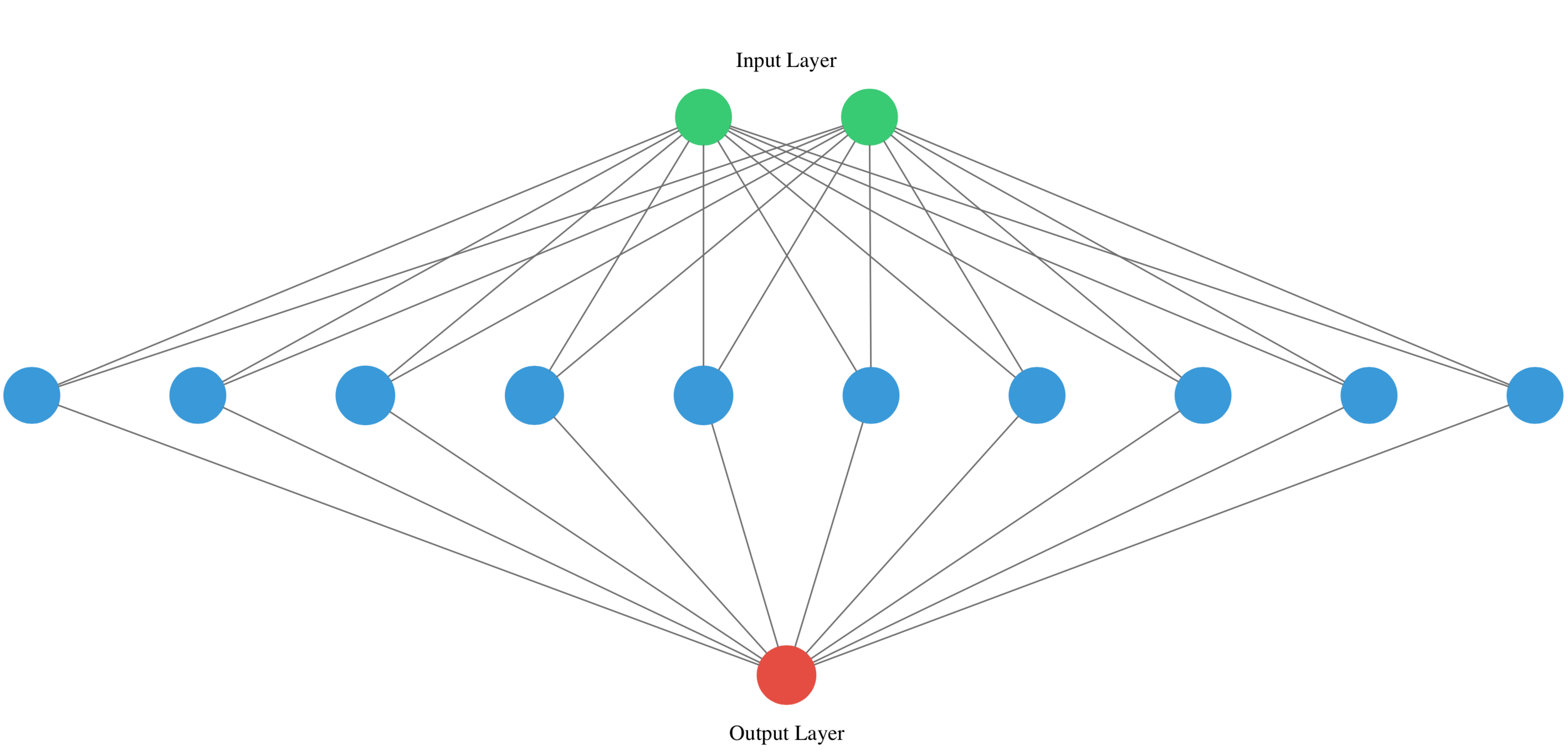
You’re going to build a simple neural network to get a feeling for how quickly it is to accomplish in Keras.
You will build a network that takes two numbers as input , passes them through a hidden layer of 10 neurons , and finally outputs a single non-constrained number .
A
non-constrained output can be obtained by avoiding setting an activation function in the output layer
. This is useful for problems like regression, when we want our output to be able to take any value.
# Import the Sequential model and Dense layer
from keras.models import Sequential
from keras.layers import Dense

# Create a Sequential model
model = Sequential()

# Add an input layer and a hidden layer with 10 neurons
model.add(Dense(10, input_shape=(2,), activation="relu"))

# Add a 1-neuron output layer
model.add(Dense(1))

# Summarise your model
model.summary()
Model: "sequential_1"
_________________________________________________________________
Layer (type)                 Output Shape              Param #
=================================================================
dense_1 (Dense)              (None, 10)                30
_________________________________________________________________
dense_2 (Dense)              (None, 1)                 11
=================================================================
Total params: 41
Trainable params: 41
Non-trainable params: 0
_________________________________________________________________
You’ve just build your first neural network with Keras, well done!
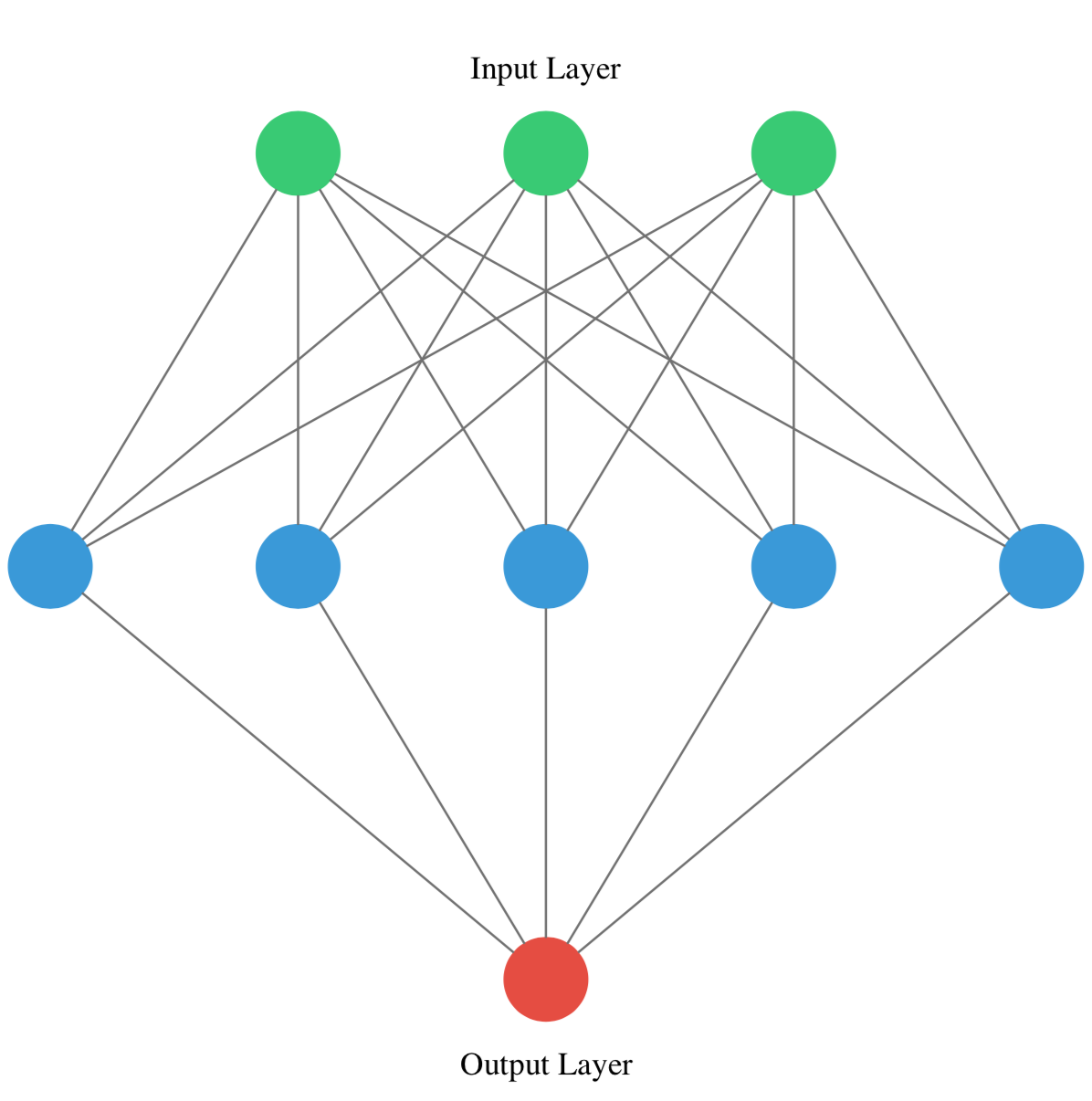
You’ve just created a neural network. Create a new one now and take some time to think about the weights of each layer. The Keras
Dense
layer and the
Sequential
model are already loaded for you to use.
This is the network you will be creating:
# Instantiate a new Sequential model
model = Sequential()

# Add a Dense layer with five neurons and three inputs
model.add(Dense(5, input_shape=(3,), activation="relu"))

# Add a final Dense layer with one neuron and no activation
model.add(Dense(1))

# Summarize your model
model.summary()
Model: "sequential_1"
_________________________________________________________________
Layer (type)                 Output Shape              Param #
=================================================================
dense_1 (Dense)              (None, 5)                 20
_________________________________________________________________
dense_2 (Dense)              (None, 1)                 6
=================================================================
Total params: 26
Trainable params: 26
Non-trainable params: 0
_________________________________________________________________
Given the
model
you just built, which answer is correct regarding the number of weights (parameters) in the
hidden layer
?
There are 20 parameters, 15 from the connection of our input layer to our hidden layer and 5 from the bias weight of each neuron in the hidden layer.
Great! You certainly know where those parameters come from!
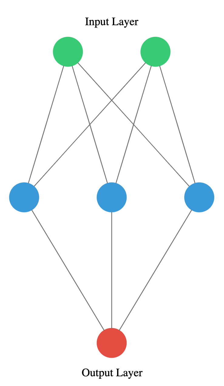
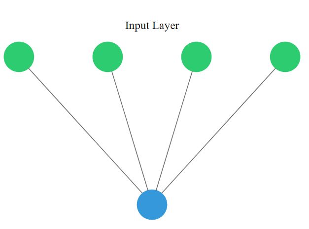
You will take on a final challenge before moving on to the next lesson. Build the network shown in the picture below. Prove your mastered Keras basics in no time!
from keras.models import Sequential
from keras.layers import Dense

# Instantiate a Sequential model
model = Sequential()

# Build the input and hidden layer
model.add(Dense(3, input_shape=(2,)))

# Add the ouput layer
model.add(Dense(1))
Perfect! You’ve shown you can already translate a visual representation of a neural network into Keras code.


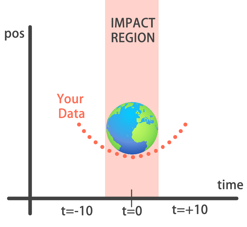
You will build a simple regression model to forecast the orbit of the meteor!
Your training data consist of measurements taken at time steps from -10 minutes before the impact region to +10 minutes after . Each time step can be viewed as an X coordinate in our graph, which has an associated position Y for the meteor at that time step.
Note that you can view this problem as approximating a quadratic function via the use of neural networks.
This data is stored in two numpy arrays: one called
time_steps
, containing the
features
, and another called
y_positions
, with the
labels
.
Feel free to look at these arrays in the console anytime, then build your model! Keras
Sequential
model and
Dense
layers are available for you to use.
# Instantiate a Sequential model
model = Sequential()

# Add a Dense layer with 50 neurons and an input of 1 neuron
model.add(Dense(50, input_shape=(1,), activation='relu'))

# Add two Dense layers with 50 neurons and relu activation
model.add(Dense(50,activation='relu'))
model.add(Dense(50,activation='relu'))

# End your model with a Dense layer and no activation
model.add(Dense(1))
You are closer to forecasting the meteor orbit! It’s important to note we aren’t using an activation function in our output layer since
y_positions
aren’t bounded and they can take any value. Your model is performing regression.
You’re going to train your first model in this course, and for a good cause!
Remember that
before training your Keras models you need to compile them
. This can be done with the
.compile()
method. The
.compile()
method takes arguments such as the
optimizer
, used for weight updating, and the
loss
function, which is what we want to minimize. Training your model is as easy as calling the
.fit()
method, passing on the
features
,
labels
and number of
epochs
to train for.
The
model
you built in the previous exercise is loaded for you to use, along with the
time_steps
and
y_positions
data.
# Compile your model
model.compile(optimizer = 'adam', loss = 'mse')

print("Training started..., this can take a while:")

# Fit your model on your data for 30 epochs
model.fit(time_steps,y_positions, epochs = 30)

# Evaluate your model
print("Final lost value:",model.evaluate(time_steps, y_positions))
Training started..., this can take a while:
Epoch 1/30

  32/2000 [..............................] - ETA: 14s - loss: 2465.2439
 928/2000 [============>.................] - ETA: 0s - loss: 1820.2874
1856/2000 [==========================>...] - ETA: 0s - loss: 1439.9186
2000/2000 [==============================] - 0s 177us/step - loss: 1369.6929
...

Epoch 30/30

  32/2000 [..............................] - ETA: 0s - loss: 0.1844
 896/2000 [============>.................] - ETA: 0s - loss: 0.2483
1696/2000 [========================>.....] - ETA: 0s - loss: 0.2292
2000/2000 [==============================] - 0s 62us/step - loss: 0.2246
  32/2000 [..............................] - ETA: 1s
1536/2000 [======================>.......] - ETA: 0s
2000/2000 [==============================] - 0s 44us/step
Final lost value: 0.14062700100243092
Amazing! You can check the console to see how the loss function decreased as epochs went by. Your model is now ready to make predictions.
You’ve already trained a
model
that approximates the orbit of the meteor approaching earth and it’s loaded for you to use.
Since you trained your model for values between -10 and 10 minutes, your model hasn’t yet seen any other values for different time steps. You will visualize how your model behaves on unseen data.
To see the source code of
plot_orbit
, type the following
print(inspect.getsource(plot_orbit))
in the console.
Remember
np.arange(x,y)
produces a range of values from
x
to
y-1
.
Hurry up, you’re running out of time!
# Predict the twenty minutes orbit
twenty_min_orbit = model.predict(np.arange(-10, 11))

# Plot the twenty minute orbit
plot_orbit(twenty_min_orbit)
# Predict the twenty minutes orbit
eighty_min_orbit = model.predict(np.arange(-40, 41))

# Plot the twenty minute orbit
plot_orbit(eighty_min_orbit)

Your model fits perfectly to the scientists trajectory for time values between -10 to +10, the region where the meteor crosses the impact region, so we won’t be hit! However, it starts to diverge when predicting for further values we haven’t trained for. This shows neural networks learn according to the data they are fed with. Data quality and diversity are very important. You’ve barely scratched the surface of what neural networks can do. Are you prepared for the next chapter?


You will practice building classification models in Keras with the Banknote Authentication dataset.
Your goal is to distinguish between real and fake dollar bills. In order to do this, the dataset comes with 4 variables:
variance
,
skewness
,
curtosis
and
entropy
. These variables are calculated by applying mathematical operations over the dollar bill images. The labels are found in the
class
variable.

The dataset is pre-loaded in your workspace as
banknotes
, let’s do some data exploration!
# Import seaborn
import seaborn as sns

# Use pairplot and set the hue to be our class
sns.pairplot(banknotes, hue='class')

# Show the plot
plt.show()

# Describe the data
print('Dataset stats: \n', banknotes.describe())

# Count the number of observations of each class
print('Observations per class: \n', banknotes['class'].value_counts())
Dataset stats:
         variance   skewness   curtosis    entropy
count  96.000000  96.000000  96.000000  96.000000
mean   -0.057791  -0.102829   0.230412   0.081497
std     1.044960   1.059236   1.128972   0.975565
min    -2.084590  -2.621646  -1.482300  -3.034187
25%    -0.839124  -0.916152  -0.415294  -0.262668
50%    -0.026748  -0.037559  -0.033603   0.394888
75%     0.871034   0.813601   0.978766   0.745212
max     1.869239   1.634072   3.759017   1.343345

Observations per class:
 real    53
fake    43
Name: class, dtype: int64

Your pairplot shows that there are variables for which the classes spread out noticeably. This gives us an intuition about our classes being separable. Let’s build a model to find out what it can do!
Now that you know what the Banknote Authentication dataset looks like, we’ll build a simple model to distinguish between real and fake bills.
You will perform binary classification by using a single neuron as an output. The input layer will have 4 neurons since we have 4 features in our dataset. The model output will be a value constrained between 0 and 1.
We will interpret this number as the probability of our input variables coming from a fake dollar bill, with 1 meaning we are certain it’s fake.
# Import the sequential model and dense layer
from keras.models import Sequential
from keras.layers import Dense

# Create a sequential model
model = Sequential()

# Add a dense layer
model.add(Dense(1, input_shape=(4,), activation='sigmoid'))

# Compile your model
model.compile(loss='binary_crossentropy', optimizer='sgd', metrics=['accuracy'])

# Display a summary of your model
model.summary()
Model: "sequential_2"
_________________________________________________________________
Layer (type)                 Output Shape              Param #
=================================================================
dense_2 (Dense)              (None, 1)                 5
=================================================================
Total params: 5
Trainable params: 5
Non-trainable params: 0
_________________________________________________________________
That was fast! Let’s use this model to make predictions!
You are now ready to train your
model
and check how well it performs when classifying new bills! The dataset has already been partitioned as
X_train
,
X_test
,
y_train
and
y_test
.
# Train your model for 20 epochs
model.fit(X_train, y_train, epochs=20)

# Evaluate your model accuracy on the test set
accuracy = model.evaluate(X_test, y_test)[1]

# Print accuracy
print('Accuracy:',accuracy)
# Accuracy: 0.8252427167105443
Alright! It looks like you are getting a high accuracy with this simple model!


You’re going to build a model that predicts who threw which dart only based on where that dart landed! (That is the dart’s x and y coordinates.)
This problem is a multi-class classification problem since each dart can only be thrown by one of 4 competitors. So classes are mutually exclusive, and therefore we can build a neuron with as many output as competitors and use the
softmax
activation function to achieve a total sum of probabilities of 1 over all competitors.
Keras
Sequential
model and
Dense
layer are already loaded for you to use.
# Instantiate a sequential model
model = Sequential()

# Add 3 dense layers of 128, 64 and 32 neurons each
model.add(Dense(128, input_shape=(2,), activation='relu'))
model.add(Dense(64, activation='relu'))
model.add(Dense(32, activation='relu'))

# Add a dense layer with as many neurons as competitors
model.add(Dense(4, activation='softmax'))

# Compile your model using categorical_crossentropy loss
model.compile(loss='categorical_crossentropy',
              optimizer='adam',
              metrics=['accuracy'])
Good job! Your models are getting deeper, just as your knowledge on neural networks!
In the console you can check that your labels,
darts.competitor
are not yet in a format to be understood by your network. They contain the names of the competitors as strings. You will first turn these competitors into unique numbers,then use the
to_categorical()
function from
keras.utils
to turn these numbers into their one-hot encoded representation.
This is useful for multi-class classification problems, since there are as many output neurons as classes and for every observation in our dataset we just want one of the neurons to be activated.
The dart’s dataset is loaded as
darts
. Pandas is imported as
pd
. Let’s prepare this dataset!
darts.head()
     xCoord    yCoord competitor
0  0.196451 -0.520341      Steve
1  0.476027 -0.306763      Susan
2  0.003175 -0.980736    Michael
3  0.294078  0.267566       Kate
4 -0.051120  0.598946      Steve

darts.info()
<class 'pandas.core.frame.DataFrame'>
RangeIndex: 800 entries, 0 to 799
Data columns (total 3 columns):
xCoord        800 non-null float64
yCoord        800 non-null float64
competitor    800 non-null object
dtypes: float64(2), object(1)
memory usage: 18.8+ KB
# Transform into a categorical variable
darts.competitor = pd.Categorical(darts.competitor)

# Assign a number to each category (label encoding)
darts.competitor = darts.competitor.cat.codes

# Print the label encoded competitors
print('Label encoded competitors: \n',darts.competitor.head())
Label encoded competitors:
 0    2
1    3
2    1
3    0
4    2
Name: competitor, dtype: int8
# Transform into a categorical variable
darts.competitor = pd.Categorical(darts.competitor)

# Assign a number to each category (label encoding)
darts.competitor = darts.competitor.cat.codes

# Import to_categorical from keras utils module
from keras.utils import to_categorical

# Use to_categorical on your labels
coordinates = darts.drop(['competitor'], axis=1)
competitors = to_categorical(darts.competitor)

# Now print the to_categorical() result
print('One-hot encoded competitors: \n',competitors)
One-hot encoded competitors:
 [[0. 0. 1. 0.]
 [0. 0. 0. 1.]
 [0. 1. 0. 0.]
 ...
 [0. 1. 0. 0.]
 [0. 1. 0. 0.]
 [0. 0. 0. 1.]]
Great! Each competitor is now a vector of length 4, full of zeroes except for the position representing her or himself.
Your model is now ready, just as your dataset. It’s time to train!
The
coordinates
and
competitors
variables you just transformed have been partitioned into
coord_train
,
competitors_train
,
coord_test
and
competitors_test
. Your
model
is also loaded. Feel free to visualize your training data or
model.summary()
in the console.
# Train your model on the training data for 200 epochs
model.fit(coord_train,competitors_train,epochs=200)

# Evaluate your model accuracy on the test data
accuracy = model.evaluate(coord_test, competitors_test)[1]

# Print accuracy
print('Accuracy:', accuracy)
# Accuracy: 0.8375
Your model just trained for 200 epochs! The accuracy on the test set is quite high. What do the predictions look like?
Your recently trained
model
is loaded for you. This model is generalizing well!, that’s why you got a high accuracy on the test set.
Since you used the
softmax
activation function, for every input of 2 coordinates provided to your model there’s an output vector of 4 numbers. Each of these numbers encodes the probability of a given dart being thrown by one of the 4 possible competitors.
When computing accuracy with the model’s
.evaluate()
method, your model takes the class with the highest probability as the prediction.
np.argmax()
can help you do this since it returns the index with the highest value in an array.
Use the collection of test throws stored in
coords_small_test
and
np.argmax()
to check this out!
# Predict on coords_small_test
preds = model.predict(coords_small_test)

# Print preds vs true values
print("{:45} | {}".format('Raw Model Predictions','True labels'))
for i,pred in enumerate(preds):
  print("{} | {}".format(pred,competitors_small_test[i]))
Raw Model Predictions                         | True labels
[0.34438723 0.00842557 0.63167274 0.01551455] | [0. 0. 1. 0.]
[0.0989717  0.00530467 0.07537904 0.8203446 ] | [0. 0. 0. 1.]
[0.33512568 0.00785374 0.28132284 0.37569773] | [0. 0. 0. 1.]
[0.8547263  0.01328656 0.11279515 0.01919206] | [1. 0. 0. 0.]
[0.3540977  0.00867271 0.6223853  0.01484426] | [0. 0. 1. 0.]
# Predict on coords_small_test
preds = model.predict(coords_small_test)

# Print preds vs true values
print("{:45} | {}".format('Raw Model Predictions','True labels'))
for i,pred in enumerate(preds):
  print("{} | {}".format(pred,competitors_small_test[i]))

# Extract the indexes of the highest probable predictions
preds = [np.argmax(pred) for pred in preds]

# Print preds vs true values
print("{:10} | {}".format('Rounded Model Predictions','True labels'))
for i,pred in enumerate(preds):
  print("{:25} | {}".format(pred,competitors_small_test[i]))
Rounded Model Predictions | True labels
                        2 | [0. 0. 1. 0.]
                        3 | [0. 0. 0. 1.]
                        3 | [0. 0. 0. 1.]
                        0 | [1. 0. 0. 0.]
                        2 | [0. 0. 1. 0.]
Well done! As you’ve seen you can easily interpret the softmax output. This can also help you spot those observations where your network is less certain on which class to predict, since you can see the probability distribution among classes.


You’re going to automate the watering of parcels by making an intelligent irrigation machine. Multi-label classification problems differ from multi-class problems in that each observation can be labeled with zero or more classes. So classes are not mutually exclusive.
To account for this behavior what we do is have an output layer with as many neurons as classes but this time, unlike in multi-class problems, each output neuron has a
sigmoid
activation function. This makes the output layer able to output a number between 0 and 1 in any of its neurons.
Keras
Sequential()
model and
Dense()
layers are preloaded. It’s time to build an intelligent irrigation machine!

# Instantiate a Sequential model
model = Sequential()

# Add a hidden layer of 64 neurons and a 20 neuron's input
model.add(Dense(64,input_shape=(20,), activation='relu'))

# Add an output layer of 3 neurons with sigmoid activation
model.add(Dense(3, activation='sigmoid'))

# Compile your model with adam and binary crossentropy loss
model.compile(optimizer='adam',
              loss='binary_crossentropy',
              metrics=['accuracy'])

model.summary()
Model: "sequential_2"
_________________________________________________________________
Layer (type)                 Output Shape              Param #
=================================================================
dense_3 (Dense)              (None, 64)                1344
_________________________________________________________________
dense_4 (Dense)              (None, 3)                 195
=================================================================
Total params: 1,539
Trainable params: 1,539
Non-trainable params: 0
_________________________________________________________________
Great! You’ve already built 3 models for 3 different problems!
An output of your multi-label
model
could look like this:
[0.76 , 0.99 , 0.66 ]
. If we round up probabilities higher than 0.5, this observation will be classified as containing all 3 possible labels
[1,1,1]
. For this particular problem, this would mean watering all 3 parcels in your field is the right thing to do given the input sensor measurements.
You will now train and predict with the
model
you just built.
sensors_train
,
parcels_train
,
sensors_test
and
parcels_test
are already loaded for you to use. Let’s see how well your machine performs!
# Train for 100 epochs using a validation split of 0.2
model.fit(sensors_train, parcels_train, epochs = 100, validation_split = 0.2)

# Predict on sensors_test and round up the predictions
preds = model.predict(sensors_test)
preds_rounded = np.round(preds)

# Print rounded preds
print('Rounded Predictions: \n', preds_rounded)

# Evaluate your model's accuracy on the test data
accuracy = model.evaluate(sensors_test, parcels_test)[1]

# Print accuracy
print('Accuracy:', accuracy)
...
Epoch 100/100

  32/1120 [..............................] - ETA: 0s - loss: 0.0439 - acc: 0.9896
1024/1120 [==========================>...] - ETA: 0s - loss: 0.0320 - acc: 0.9935
1120/1120 [==============================] - 0s 62us/step - loss: 0.0320 - acc: 0.9935 - val_loss: 0.5132 - val_acc: 0.8702

Rounded Predictions:
 [[1. 1. 0.]
 [0. 1. 0.]
 [0. 1. 0.]
 ...
 [1. 1. 0.]
 [0. 1. 0.]
 [0. 1. 1.]]

 32/600 [>.............................] - ETA: 0s
600/600 [==============================] - 0s 26us/step

Accuracy: 0.8844444648424784
Great work on automating this farm! You can see how the
validation_split
argument is useful for evaluating how your model performs as it trains.


The history callback is returned by default every time you train a model with the
.fit()
method. To access these metrics you can access the
history
dictionary inside the returned callback object and the corresponding keys.
The irrigation machine
model
you built in the previous lesson is loaded for you to train, along with its features and labels (X and y). This time you will store the model’s
history
callback and use the
validation_data
parameter as it trains.
You will plot the results stored in
history
with
plot_accuracy()
and
plot_loss()
, two simple matplotlib functions. You can check their code in the console by typing
print(inspect.getsource(plot_loss))
.
Let’s see the behind the scenes of our training!
# Train your model and save it's history
history = model.fit(X_train, y_train, epochs = 50,
                    validation_data=(X_test, y_test))

# Plot train vs test loss during training
plot_loss(history.history['loss'], history.history['val_loss'])

# Plot train vs test accuracy during training
plot_accuracy(history.history['acc'], history.history['val_acc'])


Awesome! These graphs are really useful for detecting overfitting and to know if your neural network would benefit from more training data. More on this on the next chapter!
The early stopping callback is useful since it allows for you to stop the model training if it no longer improves after a given number of epochs. To make use of this functionality you need to pass the callback inside a list to the model’s callback parameter in the
.fit()
method.
The
model
you built to detect fake dollar bills is loaded for you to train, this time with early stopping.
X_train
,
y_train
,
X_test
and
y_test
are also available for you to use.
# Import the early stopping callback
from keras.callbacks import EarlyStopping

# Define a callback to monitor val_acc
monitor_val_acc = EarlyStopping(monitor='val_acc',
                                patience=5)

# Train your model using the early stopping callback
model.fit(X_train, y_train,
          epochs=1000,
          validation_data=(X_test, y_test),
          callbacks=[monitor_val_acc])
...
Epoch 26/1000

 32/960 [>.............................] - ETA: 0s - loss: 0.2096 - acc: 0.9688
800/960 [========================>.....] - ETA: 0s - loss: 0.2079 - acc: 0.9563
960/960 [==============================] - 0s 94us/step - loss: 0.2091 - acc: 0.9531 - val_loss: 0.2116 - val_acc: 0.9417
Great! Now you won’t ever fall short of epochs!
Deep learning models can take a long time to train, especially when you move to deeper architectures and bigger datasets. Saving your model every time it improves as well as stopping it when it no longer does allows you to worry less about choosing the number of epochs to train for. You can also restore a saved model anytime.
The model training and validation data are available in your workspace as
X_train
,
X_test
,
y_train
, and
y_test
.
Use the
EarlyStopping()
and the
ModelCheckpoint()
callbacks so that you can go eat a jar of cookies while you leave your computer to work!
# Import the EarlyStopping and ModelCheckpoint callbacks
from keras.callbacks import EarlyStopping, ModelCheckpoint

# Early stop on validation accuracy
monitor_val_acc = EarlyStopping(monitor = 'val_acc', patience=3)

# Save the best model as best_banknote_model.hdf5
modelCheckpoint = ModelCheckpoint('best_banknote_model.hdf5', save_best_only = True)

# Fit your model for a stupid amount of epochs
history = model.fit(X_train, y_train,
                    epochs = 10000000,
                    callbacks = [monitor_val_acc, modelCheckpoint],
                    validation_data = (X_test, y_test))
...
Epoch 4/10000000

 32/960 [>.............................] - ETA: 0s - loss: 0.2699 - acc: 0.9688
960/960 [==============================] - 0s 59us/step - loss: 0.2679 - acc: 0.9312 - val_loss: 0.2870 - val_acc: 0.9126
This is a powerful callback combo! Now you always get the model that performed best, even if you early stopped at one that was already performing worse.


You’re going to build a model on the digits dataset , a sample dataset that comes pre-loaded with scikit learn. The digits dataset consist of 8×8 pixel handwritten digits from 0 to 9 :  You want to distinguish between each of the 10 possible digits given an image, so we are dealing with multi-class classification .
The dataset has already been partitioned into X_train , y_train , X_test , and y_test using 30% of the data as testing data. The labels are one-hot encoded vectors, so you don’t need to use Keras to_categorical() function.
Let’s build this new model !
# Instantiate a Sequential model
model = Sequential()

# Input and hidden layer with input_shape, 16 neurons, and relu
model.add(Dense(16, input_shape = (8*8,), activation = 'relu'))

# Output layer with 10 neurons (one per digit) and softmax
model.add(Dense(10, activation = 'softmax'))

# Compile your model
model.compile(optimizer = 'adam', loss = 'categorical_crossentropy', metrics = ['accuracy'])

# Test if your model works and can process input data
print(model.predict(X_train))
Great! Predicting on training data inputs before training can help you quickly check that your model works as expected.
Let’s train the model you just built and plot its learning curve to check out if it’s overfitting! You can make use of loaded function plot_loss() to plot training loss against validation loss, you can get both from the history callback.
If you want to inspect the plot_loss() function code, paste this in the console: print(inspect.getsource(plot_loss))
# Train your model for 60 epochs, using X_test and y_test as validation data
h_callback = model.fit(X_train, y_train, epochs=60, validation_data=(X_test, y_test), verbose=0)

# Extract from the history object loss and val_loss to plot the learning curve
plot_loss(h_callback.history['loss'], h_callback.history['val_loss'])

Just by looking at the overall picture, do you think the learning curve shows this model is overfitting after having trained for 60 epochs?
No, the test loss is not getting higher as the epochs go by.
Awesome choice! This graph doesn’t show overfitting but convergence. It looks like your model has learned all it could from the data and it no longer improves.
It’s time to check whether the digits dataset model you built benefits from more training examples!
In order to keep code to a minimum, various things are already initialized and ready to use:
modelyou just built.X_train, y_train, X_test, and y_test.initial_weights of your model, saved after using model.get_weights().training_sizes.EarlyStopping callback monitoring loss: early_stop.train_accs and test_accs.Train your model on the different training sizes and evaluate the results on X_test . End by plotting the results with plot_results().
The full code for this exercise can be found on the slides!
train_sizes
array([ 125,  502,  879, 1255])
for size in training_sizes:
    # Get a fraction of training data (we only care about the training data)
    X_train_frac, y_train_frac = X_train[:size], y_train[:size]

    # Reset the model to the initial weights and train it on the new training data fraction
    model.set_weights(initial_weights)
    model.fit(X_train_frac, y_train_frac, epochs=50, callbacks=[early_stop])

    # Evaluate and store both: the training data fraction and the complete test set results
    train_accs.append(model.evaluate(X_train_frac, y_train_frac)[1])
    test_accs.append(model.evaluate(X_test, y_test)[1])

# Plot train vs test accuracies
plot_results(train_accs, test_accs)

Great job, that was a lot of code to understand! The results shows that your model would not benefit a lot from more training data, since the test set is starting to flatten in accuracy already.


tanh(hyperbolic tangent)
The sigmoid() , tanh() , ReLU() , and leaky_ReLU() functions have been defined and ready for you to use. Each function receives an input number X and returns its corresponding Y value.
Which of the statements below is false ?
sigmoid() takes a value of 0.5 when X = 0 whilst tanh() takes a value of 0 .leaky-ReLU() takes a value of -0.01 when X = -1 whilst ReLU() takes a value of 0 .sigmoid() and tanh() both take values close to -1 for big negative numbers.(false)**Great! For big negative numbers the sigmoid approaches 0 not -1 whilst the tanh() does take values close to -1 .
Comparing activation functions involves a bit of coding, but nothing you can’t do!
You will try out different activation functions on the multi-label model you built for your irrigation machine in chapter 2. The function get_model() returns a copy of this model and applies the activation function, passed on as a parameter, to its hidden layer.
You will build a loop that goes through several activation functions, generates a new model for each and trains it. Storing the history callback in a dictionary will allow you to compare and visualize which activation function performed best in the next exercise!
# Set a seed
np.random.seed(27)

# Activation functions to try
activations = ['relu', 'leaky_relu', 'sigmoid', 'tanh']

# Loop over the activation functions
activation_results = {}

for act in activations:
  # Get a new model with the current activation
  model = get_model(act_function=act)
  # Fit the model and store the history results
  h_callback = model.fit(X_train, y_train, validation_data=(X_test,y_test), epochs=20, verbose=0)
  activation_results[act] = h_callback
Finishing with relu ...
Finishing with leaky_relu ...
Finishing with sigmoid ...
Finishing with tanh ...
Awesome job! You’ve trained 4 models with 4 different activation functions, let’s see how well they performed!
The code used in the previous exercise has been executed to obtain the activation_results with the difference that 100 epochs instead of 20 are used. That way you’ll have more epochs to further compare how the training evolves per activation function.
For every history callback of each activation function in activation_results :
history.history['val_loss'] has been extracted.history.history['val_acc'] has been extracted.val_loss_per_function and val_acc_per_function .Pandas is also loaded for you to use as pd . Let’s plot some quick comparison validation loss and accuracy charts with pandas!
# Create a dataframe from val_loss_per_function
val_loss= pd.DataFrame(val_loss_per_function)

# Call plot on the dataframe
val_loss.plot()
plt.show()

# Create a dataframe from val_acc_per_function
val_acc = pd.DataFrame(val_acc_per_function)

# Call plot on the dataframe
val_acc.plot()
plt.show()


You’ve seen models are usually trained in batches of a fixed size. The smaller a batch size, the more weight updates per epoch, but at a cost of a more unstable gradient descent. Specially if the batch size is too small and it’s not representative of the entire training set.
Let’s see how different batch sizes affect the accuracy of a binary classification model that separates red from blue dots.
You’ll use a batch size of one, updating the weights once per sample in your training set for each epoch. Then you will use the entire dataset, updating the weights only once per epoch.
# Get a fresh new model with get_model
model = get_model()

# Train your model for 5 epochs with a batch size of 1
model.fit(X_train, y_train, epochs=5, batch_size=1)
print("\n The accuracy when using a batch of size 1 is: ",
      model.evaluate(X_test, y_test)[1])
# The accuracy when using a batch of size 1 is:  0.9733333333333334
model = get_model()

# Fit your model for 5 epochs with a batch of size the training set
model.fit(X_train, y_train, epochs=5, batch_size=X_train.shape[0])
print("\n The accuracy when using the whole training set as a batch was: ",
      model.evaluate(X_test, y_test)[1])
# The accuracy when using the whole training set as a batch was:  0.553333334128062
Remember the digits dataset you trained in the first exercise of this chapter?
A multi-class classification problem that you solved using softmax and 10 neurons in your output layer.
You will now build a new deeper model consisting of 3 hidden layers of 50 neurons each, using batch normalization in between layers. The kernel_initializer parameter is used to initialize weights in a similar way.
# Import batch normalization from keras layers
from keras.layers import BatchNormalization

# Build your deep network
batchnorm_model = Sequential()
batchnorm_model.add(Dense(50, input_shape=(64,), activation='relu', kernel_initializer='normal'))
batchnorm_model.add(BatchNormalization())
batchnorm_model.add(Dense(50, activation='relu', kernel_initializer='normal'))
batchnorm_model.add(BatchNormalization())
batchnorm_model.add(Dense(50, activation='relu', kernel_initializer='normal'))
batchnorm_model.add(BatchNormalization())
batchnorm_model.add(Dense(10, activation='softmax', kernel_initializer='normal'))

# Compile your model with sgd
batchnorm_model.compile(optimizer='sgd', loss='categorical_crossentropy', metrics=['accuracy'])
Congratulations! That was a deep model indeed. Let’s compare how it performs against this very same model without batch normalization!
Batch normalization tends to increase the learning speed of our models and make their learning curves more stable. Let’s see how two identical models with and without batch normalization compare.
The model you just built batchnorm_model is loaded for you to use. An exact copy of it without batch normalization: standard_model , is available as well. You can check their summary() in the console. X_train , y_train , X_test , and y_test are also loaded so that you can train both models.
You will compare the accuracy learning curves for both models plotting them with compare_histories_acc() .
You can check the function pasting print(inspect.getsource(compare_histories_acc)) in the console.
# Train your standard model, storing its history callback
h1_callback = standard_model.fit(X_train, y_train, validation_data=(X_test,y_test), epochs=10, verbose=0)

# Train the batch normalized model you recently built, store its history callback
h2_callback = batchnorm_model.fit(X_train, y_train, validation_data=(X_test,y_test), epochs=10, verbose=0)

# Call compare_histories_acc passing in both model histories
compare_histories_acc(h1_callback, h2_callback)

Outstanding! You can see that for this deep model batch normalization proved to be useful, helping the model obtain high accuracy values just over the first 10 training epochs.


Let’s tune the hyperparameters of a binary classification model that does well classifying the breast cancer dataset .
You’ve seen that the first step to turn a model into a sklearn estimator is to build a function that creates it. This function is important since you can play with the parameters it receives to achieve the different models you’d like to try out.
Build a simple create_model() function that receives a learning rate and an activation function as parameters. The Adam optimizer has been imported as an object from keras.optimizers so that you can change its learning rate parameter.
# Creates a model given an activation and learning rate
def create_model(learning_rate, activation):

  	# Create an Adam optimizer with the given learning rate
  	opt = Adam(lr = learning_rate)

  	# Create your binary classification model
  	model = Sequential()
  	model.add(Dense(128, input_shape = (30,), activation = activation))
  	model.add(Dense(256, activation = activation))
  	model.add(Dense(1, activation = 'sigmoid'))

  	# Compile your model with your optimizer, loss, and metrics
  	model.compile(optimizer = opt, loss = 'binary_crossentropy', metrics = ['accuracy'])
  	return model
Well done! With this function ready you can now create a sklearn estimator and perform hyperparameter tuning!
It’s time to try out different parameters on your model and see how well it performs!
The create_model() function you built in the previous exercise is loaded for you to use.
Since fitting the RandomizedSearchCV would take too long, the results you’d get are printed in the show_results() function. You could try random_search.fit(X,y) in the console yourself to check it does work after you have built everything else, but you will probably timeout your exercise (so copy your code first if you try it!).
You don’t need to use the optional epochs and batch_size parameters when building your KerasClassifier since you are passing them as params to the random search and this works as well.
# Import KerasClassifier from keras scikit learn wrappers
from keras.wrappers.scikit_learn import KerasClassifier

# Create a KerasClassifier
model = KerasClassifier(build_fn = create_model)

# Define the parameters to try out
params = {'activation': ['relu', 'tanh'], 'batch_size': [32, 128, 256],
          'epochs': [50, 100, 200], 'learning_rate': [0.1, 0.01, 0.001]}

# Create a randomize search cv object passing in the parameters to try
random_search = RandomizedSearchCV(model, param_distributions = params, cv = KFold(3))

# Running random_search.fit(X,y) would start the search,but it takes too long!
show_results()
Best: 0.975395 using {learning_rate: 0.001, epochs: 50, batch_size: 128, activation: relu}
 0.956063 (0.013236) with: {learning_rate: 0.1, epochs: 200, batch_size: 32, activation: tanh}
 0.970123 (0.019838) with: {learning_rate: 0.1, epochs: 50, batch_size: 256, activation: tanh}
 0.971880 (0.006524) with: {learning_rate: 0.01, epochs: 100, batch_size: 128, activation: tanh}
 0.724077 (0.072993) with: {learning_rate: 0.1, epochs: 50, batch_size: 32, activation: relu}
 0.588752 (0.281793) with: {learning_rate: 0.1, epochs: 100, batch_size: 256, activation: relu}
 0.966608 (0.004892) with: {learning_rate: 0.001, epochs: 100, batch_size: 128, activation: tanh}
 0.952548 (0.019734) with: {learning_rate: 0.1, epochs: 50, batch_size: 256, activation: relu}
 0.971880 (0.006524) with: {learning_rate: 0.001, epochs: 200, batch_size: 128, activation: relu}
 0.968366 (0.004239) with: {learning_rate: 0.01, epochs: 100, batch_size: 32, activation: relu}
 0.910369 (0.055824) with: {learning_rate: 0.1, epochs: 100, batch_size: 128, activation: relu}
That was great! I’m glad that the server is still working. Now that we have a better idea of which parameters are performing best, let’s use them!
Time to train your model with the best parameters found: 0.001 for the learning rate , 50 epochs , a 128 batch_size and relu activations .
The create_model() function has been redefined so that it now creates a model with those parameters. X and y are loaded for you to use as features and labels.
In this exercise you do pass the best epochs and batch size values found for your model to the KerasClassifier object so that they are used when performing cross validation.
End this chapter by training an awesome tuned model on the breast cancer dataset !
# Import KerasClassifier from keras wrappers
from keras.wrappers.scikit_learn import KerasClassifier

# Create a KerasClassifier
model = KerasClassifier(build_fn = create_model(learning_rate = 0.001, activation = 'relu'), epochs = 50,
             batch_size = 128, verbose = 0)

# Calculate the accuracy score for each fold
kfolds = cross_val_score(model, X, y, cv = 3)

# Print the mean accuracy
print('The mean accuracy was:', kfolds.mean())

# Print the accuracy standard deviation
print('With a standard deviation of:', kfolds.std())
The mean accuracy was: 0.9718834066666666
With a standard deviation of: 0.002448915612216046
Amazing! Now you can more reliably test out different parameters on your networks and find better models!


If you have already built a model, you can use the
model.layers
and the
keras.backend
to build functions that, provided with a valid input tensor, return the corresponding output tensor.
This is a useful tool when trying to understand what is going on inside the layers of a neural network.
For instance, if you get the input and output from the first layer of a network, you can build an
inp_to_out
function that returns the result of carrying out forward propagation through only the first layer for a given input tensor.
So that’s what you’re going to do right now!
X_test
from the
Banknote Authentication
dataset and its
model
are preloaded. Type
model.summary()
in the console to check it.
# Import keras backend
import keras.backend as K

# Input tensor from the 1st layer of the model
inp = model.layers[0].input

# Output tensor from the 1st layer of the model
out = model.layers[0].output

# Define a function from inputs to outputs
inp_to_out = K.function([inp],[out])

# Print the results of passing X_test through the 1st layer
print(inp_to_out([X_test]))
[array([[7.77682841e-01, 0.00000000e+00],
       [0.00000000e+00, 0.00000000e+00],
       [0.00000000e+00, 1.50813460e+00],
       [0.00000000e+00, 1.34600031e+00],
...
Nice job! Let’s use this function for something more interesting.
Neurons learn by updating their weights to output values that help them distinguish between the input classes. So put on your gloves because you’re going to perform brain surgery!
You will make use of the
inp_to_out()
function you just built to visualize the output of two neurons in the first layer of the
Banknote Authentication
model
as epochs go by. Plotting the outputs of both of these neurons against each other will show you the difference in output depending on whether each bill was real or fake.
The
model
you built in chapter 2 is ready for you to use, just like
X_test
and
y_test
. Copy
print(inspect.getsource(plot))
in the console if you want to check
plot()
.
You’re performing heavy duty, once it’s done, take a look at the graphs to watch the separation live!
print(inspect.getsource(plot))
def plot():
  fig, ax = plt.subplots()
  plt.scatter(layer_output[:, 0], layer_output[:, 1],c=y_test,edgecolors='none')
  plt.title('Epoch: {}, Test Acc: {:3.1f} %'.format(i+1, test_accuracy * 100.0))
  plt.show()
for i in range(0, 21):
  	# Train model for 1 epoch
    h = model.fit(X_train, y_train, batch_size=16, epochs=1,verbose=0)
    if i%4==0:
      # Get the output of the first layer
      layer_output = inp_to_out([X_test])[0]

      # Evaluate model accuracy for this epoch
      test_accuracy = model.evaluate(X_test, y_test)[1]

      # Plot 1st vs 2nd neuron output
      plot()


That took a while! If you take a look at the graphs you can see how the neurons are learning to spread out the classes during training. Click in between graphs fast, it’s like a movie!
Autoencoders have several interesting applications like anomaly detection or image denoising. They aim at producing an output identical to its inputs. The input will be compressed into a lower dimensional space, encoded . The model then learns to decode it back to its original form.
You will encode and decode the MNIST dataset of handwritten digits, the hidden layer will encode a 32-dimensional representation of the image, which originally consists of 784 pixels.
The
Sequential
model and
Dense
layers are ready for you to use.
Let’s build an autoencoder!
# Start with a sequential model
autoencoder = Sequential()

# Add a dense layer with input the original image pixels and neurons the encoded representation
autoencoder.add(Dense(32, input_shape=(784, ), activation="relu"))

# Add an output layer with as many neurons as the orginal image pixels
autoencoder.add(Dense(784, activation="sigmoid"))

# Compile your model with adadelta
autoencoder.compile(optimizer='adadelta', loss='binary_crossentropy')

# Summarize your model structure
autoencoder.summary()
Model: "sequential_1"
_________________________________________________________________
Layer (type)                 Output Shape              Param #
=================================================================
dense_1 (Dense)              (None, 32)                25120
_________________________________________________________________
dense_2 (Dense)              (None, 784)               25872
=================================================================
Total params: 50,992
Trainable params: 50,992
Non-trainable params: 0
_________________________________________________________________
Great start! Your model is now ready. Let’s see what you can do with it!
Okay, you have just built an
autoencoder
model. Let’s see how it handles a more challenging task.
First, you will build a model that encodes images, and you will check how different digits are represented with
show_encodings()
. You can change the
number
parameter of this function to check other digits in the console.
Then, you will apply your
autoencoder
to noisy images from
MNIST
, it should be able to clean the noisy artifacts.
X_test_noise
is loaded in your workspace. The digits in this data look like this:

Apply the power of the autoencoder!
# Build your encoder by using the first layer of your autoencoder
encoder = Sequential()
encoder.add(autoencoder.layers[0])

# Encode the noisy images and show the encodings for your favorite number [0-9]
encodings = encoder.predict(X_test_noise)
show_encodings(encodings, number = 1)

# Predict on the noisy images with your autoencoder
decoded_imgs = autoencoder.predict(X_test_noise)

# Plot noisy vs decoded images
compare_plot(X_test_noise, decoded_imgs)
Amazing! The noise is gone now! You could get a better reconstruction by using a convolutional autoencoder.


Building a CNN model in Keras isn’t much more difficult than building any of the models you’ve already built throughout the course! You just need to make use of convolutional layers.
You’re going to build a shallow convolutional
model
that classifies the
MNIST
dataset of digits. The same one you de-noised with your autoencoder!. The images are 28×28 pixels and just have one channel.
Go ahead and build this small convolutional model!
# Import the Conv2D and Flatten layers and instantiate model
from keras.layers import Conv2D,Flatten
model = Sequential()

# Add a convolutional layer of 32 filters of size 3x3
model.add(Conv2D(32, input_shape=(28, 28, 1), kernel_size=3, activation='relu'))

# Add a convolutional layer of 16 filters of size 3x3
model.add(Conv2D(16, kernel_size=3, activation='relu'))

# Flatten the previous layer output
model.add(Flatten())

# Add as many outputs as classes with softmax activation
model.add(Dense(10, activation = 'softmax'))
Well done! You can see that the key concepts are the same, you just have to use new layers!
Inspecting the activations of a convolutional layer is a cool thing. You have to do it at least once in your lifetime!
To do so, you will build a new model with the Keras
Model
object, which takes in a list of inputs and a list of outputs. The output you will provide to this new model is the first convolutional layer outputs when given an
MNIST
digit as input image.
The convolutional
model
you built in the previous exercise has already been trained for you. You can check it with
model.summary()
in the console.
Let’s look at a couple convolutional masks that were learned in the first convolutional layer of this model!
# Obtain a reference to the outputs of the first layer
first_layer_output = model.layers[0].output

# Build a model using the model's input and the first layer output
first_layer_model = Model(inputs = model.layers[0].input, outputs = first_layer_output)

# Use this model to predict on X_test
activations = first_layer_model.predict(X_test)

# Plot the activations of first digit of X_test for the 15th filter
axs[0].matshow(activations[0,:,:,14], cmap = 'viridis')

# Do the same but for the 18th filter now
axs[1].matshow(activations[0,:,:,17], cmap = 'viridis')
plt.show()

Hurrah! Each neuron filter of the first layer learned a different convolution. The 15th filter (a.k.a convolutional mask) learned to detect horizontal traces in your digits. On the other hand, filter 18th seems to be checking for vertical traces.
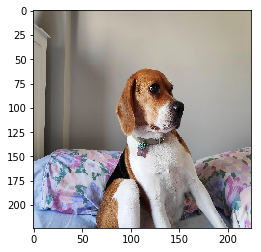
When using an already trained model like ResNet50 , we need to make sure that we fit the network the way it was originally trained. So if we want to use a trained model on our custom images, these images need to have the same dimensions as the one used in the original model.
The original ResNet50 model was trained with images of size 224×224 pixels and a number of preprocessing operations; like the subtraction of the mean pixel value in the training set for all training images.
You will go over these preprocessing steps as you prepare this dog’s (named Ivy) image into one that can be classified by
ResNet50
.

# Import image and preprocess_input
from keras.preprocessing import image
from keras.applications.resnet50 import preprocess_input

# Load the image with the right target size for your model
img = image.load_img(img_path, target_size=(224, 224))

# Turn it into an array
img_array = image.img_to_array(img)

# Expand the dimensions of the image, this is so that it fits the expected model input format
img_expanded = np.expand_dims(img_array, axis = 0)

# Pre-process the img in the same way original images were
img_ready = preprocess_input(img_expanded)
Alright! Ivy is now ready for ResNet50. Do you know this dog’s breed? Let’s see what this model thinks it is!
Okay, so Ivy’s picture is ready to be used by
ResNet50
. It is stored in
img_ready
and now looks like this:
ResNet50 is a model trained on the Imagenet dataset that is able to distinguish between 1000 different objects. ResNet50 is a deep model with 50 layers, you can check it in 3D here .
ResNet50
and
decode_predictions
have both been imported from
keras.applications.resnet50
for you.
It’s time to use this trained model to find out Ivy’s breed!
# Instantiate a ResNet50 model with 'imagenet' weights
model = ResNet50(weights='imagenet')

# Predict with ResNet50 on your already processed img
preds = model.predict(img_ready)

# Decode the first 3 predictions
print('Predicted:', decode_predictions(preds, top=3)[0])
Predicted: [(‘n02088364’, ‘beagle’, 0.8280003), (‘n02089867’, ‘Walker_hound’, 0.12915272), (‘n02089973’, ‘English_foxhound’, 0.03711732)]
Amazing! Now you know Ivy is a Beagle and that deep learning models that have already been trained for you are easy to use!


During the following exercises you will build an LSTM model that is able to predict the next word using a small text dataset. This dataset consist of cleaned quotes from the
The Lord of the Ring
movies. You can find them in the
text
variable.
You will turn this
text
into
sequences
of
length 4
and make use of the Keras
Tokenizer
to prepare the features and labels for your model!
The Keras
Tokenizer
is already imported for you to use. It assigns a unique number to each unique word, and stores the mappings in a dictionary. This is important since the model deals with numbers but we later will want to decode the output numbers back into words.
You’re working with this small chunk of The Lord of The Ring quotes:
text
'it is not the strength of the body but the strength of the spirit it is useless to meet revenge with revenge it will heal nothing even the smallest person can change the course of history all we have to decide is what to do with the time that is given us the burned hand teaches best after that advice about fire goes to the heart'
# Split text into an array of words
words = text.split()

# Make sentences of 4 words each, moving one word at a time
sentences = []
for i in range(4, len(words)):
  sentences.append(' '.join(words[i-4:i]))

# Instantiate a Tokenizer, then fit it on the sentences
tokenizer = Tokenizer()
tokenizer.fit_on_texts(sentences)

# Turn sentences into a sequence of numbers
sequences = tokenizer.texts_to_sequences(sentences)
print("Sentences: \n {} \n Sequences: \n {}".format(sentences[:5],sequences[:5]))
Lines:
 ['it is not the', 'is not the strength', 'not the strength of', 'the strength of the', 'strength of the body']
 Sequences:
 [[5, 2, 42, 1], [2, 42, 1, 6], [42, 1, 6, 4], [1, 6, 4, 1], [6, 4, 1, 10]]
Great! Your lines are now sequences of numbers, check that identical words are assigned the same number.
You’ve already prepared your sequences of text, with each of the sequences consisting of four words. It’s time to build your LSTM model!
Your model will be trained on the first three words of each sequence, predicting the 4th one. You are going to use an
Embedding
layer that will essentially learn to turn words into vectors. These vectors will then be passed to a simple
LSTM
layer. Our output is a
Dense
layer with as many neurons as words in the vocabulary and
softmax
activation. This is because we want to obtain the highest probable next word out of all possible words.
The size of the vocabulary of words (the unique number of words) is stored in
vocab_size
.
# Import the Embedding, LSTM and Dense layer
from keras.layers import Embedding, LSTM, Dense

model = Sequential()

# Add an Embedding layer with the right parameters
model.add(Embedding(input_dim=vocab_size, output_dim=8, input_length=3))

# Add a 32 unit LSTM layer
model.add(LSTM(32))

# Add a hidden Dense layer of 32 units and an output layer of vocab_size with softmax
model.add(Dense(32, activation='relu'))
model.add(Dense(vocab_size, activation='softmax'))
model.summary()
Model: "sequential_1"
_________________________________________________________________
Layer (type)                 Output Shape              Param #
=================================================================
embedding_1 (Embedding)      (None, 3, 8)              352
_________________________________________________________________
lstm_1 (LSTM)                (None, 32)                5248
_________________________________________________________________
dense_1 (Dense)              (None, 32)                1056
_________________________________________________________________
dense_2 (Dense)              (None, 44)                1452
=================================================================
Total params: 8,108
Trainable params: 8,108
Non-trainable params: 0
_________________________________________________________________
That’s a nice looking model you’ve built! You’ll see that this model is powerful enough to learn text relationships. Specially because we aren’t using a lot of text in this tiny example.
Your LSTM
model
has already been trained for you so that you don’t have to wait. It’s time to
define a function
that decodes its predictions.
Since you are predicting on a model that uses the softmax function,
argmax()
is used to obtain the position of the output layer with the highest probability, that is the index representing the most probable next word.
The
tokenizer
you previously created and fitted, is loaded for you. You will be making use of its internal
index_word
dictionary to turn the model’s next word prediction (which is an integer) into the actual written word it represents.
You’re very close to experimenting with your model!
def predict_text(test_text):
  if len(test_text.split())!=3:
    print('Text input should be 3 words!')
    return False

  # Turn the test_text into a sequence of numbers
  test_seq = tokenizer.texts_to_sequences([test_text])
  test_seq = np.array(test_seq)

  # Get the model's next word prediction by passing in test_seq
  pred = model.predict(test_seq).argmax(axis = 1)[0]

  # Return the word associated to the predicted index
  return tokenizer.index_word[pred]
Great job! It’s finally time to try out your model to see how well it does!
The function you just built,
predict_text()
, is ready to use.
Try out these strings on your LSTM model:
'meet revenge with''the course of''strength of the'Which sentence could be made with the word output from the sentences above?
A worthless gnome is king
*Revenge is your history and spirit *
Take a sword and ride to Florida
predict_text('meet revenge with')
'revenge'

predict_text('the course of')
'history'

predict_text('strength of the')
'spirit'


Thank you for reading and hope you’ve learned a lot.