
This is the memo of the 25th course of ‘Data Scientist with Python’ track.
You can find the original course HERE .


#### Coding the forward propagation algorithm
In this exercise, you’ll write code to do forward propagation (prediction) for your first neural network:

Each data point is a customer. The first input is how many accounts they have, and the second input is how many children they have. The model will predict how many transactions the user makes in the next year.
You will use this data throughout the first 2 chapters of this course.
input_data
# array([3, 5])

weights
 # {'node_0': array([2, 4]), 'node_1': array([ 4, -5]), 'output': array([2, 7])}
input_data * weights['node_0']
# array([ 6, 20])

np.array([3, 5]) * np.array([2, 4])
# array([ 6, 20])

(input_data * weights['node_0']).sum()
# 26
# Calculate node 0 value: node_0_value
node_0_value = (input_data * weights['node_0']).sum()

# Calculate node 1 value: node_1_value
node_1_value = (input_data * weights['node_1']).sum()

# Put node values into array: hidden_layer_outputs
hidden_layer_outputs = np.array([node_0_value, node_1_value])

# Calculate output: output
output = (hidden_layer_outputs * weights['output']).sum()

# Print output
print(output)

#    -39
It looks like the network generated a prediction of
-39
.


#### The Rectified Linear Activation Function
An “activation function” is a function applied at each node. It converts the node’s input into some output.
The rectified linear activation function (called ReLU ) has been shown to lead to very high-performance networks. This function takes a single number as an input, returning 0 if the input is negative, and the input if the input is positive.
Here are some examples:
relu(3) = 3
relu(-3) = 0
def relu(input):
    '''Define your relu activation function here'''
    # Calculate the value for the output of the relu function: output
    output = max(input, 0)

    # Return the value just calculated
    return(output)

# Calculate node 0 value: node_0_output
node_0_input = (input_data * weights['node_0']).sum()
node_0_output = relu(node_0_input)

# Calculate node 1 value: node_1_output
node_1_input = (input_data * weights['node_1']).sum()
node_1_output = relu(node_1_input)

# Put node values into array: hidden_layer_outputs
hidden_layer_outputs = np.array([node_0_output, node_1_output])

# Calculate model output (do not apply relu)
model_output = (hidden_layer_outputs * weights['output']).sum()

# Print model output
print(model_output)

# 52
You predicted 52 transactions. Without this activation function, you would have predicted a negative number!
The real power of activation functions will come soon when you start tuning model weights.
#### Applying the network to many observations/rows of data
input_data
[array([3, 5]), array([ 1, -1]), array([0, 0]), array([8, 4])]

weights
{'node_0': array([2, 4]), 'node_1': array([ 4, -5]), 'output': array([2, 7])}
def relu(input):
    '''Define relu activation function'''
    return(max(input, 0))

# Define predict_with_network()
def predict_with_network(input_data_row, weights):

    # Calculate node 0 value
    node_0_input = (input_data_row * weights['node_0']).sum()
    node_0_output = relu(node_0_input)

    # Calculate node 1 value
    node_1_input = (input_data_row * weights['node_1']).sum()
    node_1_output = relu(node_1_input)

    # Put node values into array: hidden_layer_outputs
    hidden_layer_outputs = np.array([node_0_output, node_1_output])

    # Calculate model output
    input_to_final_layer = (hidden_layer_outputs * weights['output']).sum()
    model_output = relu(input_to_final_layer)

    # Return model output
    return(model_output)


# Create empty list to store prediction results
results = []
for input_data_row in input_data:
    # Append prediction to results
    results.append(predict_with_network(input_data_row, weights))

# Print results
print(results)

# [52, 63, 0, 148]


#### Forward propagation in a deeper network
You now have a model with 2 hidden layers. The values for an input data point are shown inside the input nodes. The weights are shown on the edges/lines. What prediction would this model make on this data point?
Assume the activation function at each node is the identity function . That is, each node’s output will be the same as its input. So the value of the bottom node in the first hidden layer is -1, and not 0, as it would be if the ReLU activation function was used.
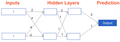
| Hidden Layer 1 | Hidden Layer 2 | Prediction | | 6 | -1 | | | | | 0 | | -1 | 5 | |
#### Multi-layer neural networks
In this exercise, you’ll write code to do forward propagation for a neural network with 2 hidden layers. Each hidden layer has two nodes.
input_data
array([3, 5])

weights
{'node_0_0': array([2, 4]),
 'node_0_1': array([ 4, -5]),
 'node_1_0': array([-1,  2]),
 'node_1_1': array([1, 2]),
 'output': array([2, 7])}
def predict_with_network(input_data):
    # Calculate node 0 in the first hidden layer
    node_0_0_input = (input_data * weights['node_0_0']).sum()
    node_0_0_output = relu(node_0_0_input)

    # Calculate node 1 in the first hidden layer
    node_0_1_input = (input_data * weights['node_0_1']).sum()
    node_0_1_output = relu(node_0_1_input)

    # Put node values into array: hidden_0_outputs
    hidden_0_outputs = np.array([node_0_0_output, node_0_1_output])

    # Calculate node 0 in the second hidden layer
    node_1_0_input = (hidden_0_outputs * weights['node_1_0']).sum()
    node_1_0_output = relu(node_1_0_input)

    # Calculate node 1 in the second hidden layer
    node_1_1_input = (hidden_0_outputs * weights['node_1_1']).sum()
    node_1_1_output = relu(node_1_1_input)

    # Put node values into array: hidden_1_outputs
    hidden_1_outputs = np.array([node_1_0_output, node_1_1_output])

    # Calculate model output: model_output
    model_output = (hidden_1_outputs * weights['output']).sum()

    # Return model_output
    return(model_output)

output = predict_with_network(input_data)
print(output)

# 182
#### Representations are learned
How are the weights that determine the features/interactions in Neural Networks created?
The model training process sets them to optimize predictive accuracy.
#### Levels of representation
Which layers of a model capture more complex or “higher level” interactions?
The last layers capture the most complex interactions.
#### Calculating model errors
What is the error (predicted – actual) for the following network when the input data is [3, 2] and the actual value of the target (what you are trying to predict) is 5?
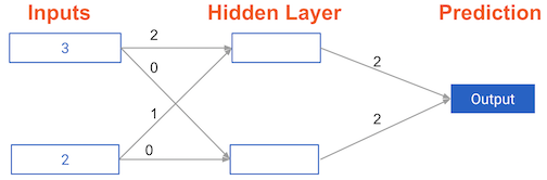
prediction = (32 + 21) * 2 + (30 + 20)*2
=16
error = 16 – 5 = 11
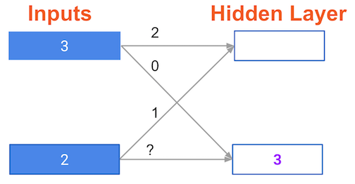
#### Understanding how weights change model accuracy
Imagine you have to make a prediction for a single data point. The actual value of the target is 7. The weight going from
node_0
to the output is 2, as shown below.
If you increased it slightly, changing it to 2.01, would the predictions become more accurate, less accurate, or stay the same?
prediction_before = 16
error_before = 16 – 7 = 9
prediction_after = (32.01 + 21) * 2 + (30 + 20)*2
=16.x
error_after = 9.x
Increasing the weight to
2.01
would increase the resulting error from
9
to
9.08
, making the predictions
less
accurate.
#### Coding how weight changes affect accuracy
Now you’ll get to change weights in a real network and see how they affect model accuracy!

Have a look at the following neural network:
weights_0weights_0weights_1target_actual
# The data point you will make a prediction for
input_data = np.array([0, 3])

# Sample weights
weights_0 = {'node_0': [2, 1],
             'node_1': [1, 2],
             'output': [1, 1]
            }

# The actual target value, used to calculate the error
target_actual = 3

# Make prediction using original weights
model_output_0 = predict_with_network(input_data, weights_0)

# Calculate error: error_0
error_0 = model_output_0 - target_actual

# Create weights that cause the network to make perfect prediction (3): weights_1
weights_1 = {'node_0': [2, 1],
             'node_1': [1, 2],
             'output': [1, 0]
            }

# Make prediction using new weights: model_output_1
model_output_1 = predict_with_network(input_data, weights_1)

# Calculate error: error_1
error_1 = model_output_1 - target_actual

# Print error_0 and error_1
print(error_0)
print(error_1)

# 6
# 0
#### Scaling up to multiple data points
You’ve seen how different weights will have different accuracies on a single prediction. But usually, you’ll want to measure model accuracy on many points.
You’ll now write code to compare model accuracies for two different sets of weights, which have been stored as
weights_0
and
weights_1
.
input_data
[array([0, 3]), array([1, 2]), array([-1, -2]), array([4, 0])]

target_actuals
[1, 3, 5, 7]

weights_0
{'node_0': array([2, 1]), 'node_1': array([1, 2]), 'output': array([1, 1])}

weights_1
{'node_0': array([2, 1]),
 'node_1': array([1. , 1.5]),
 'output': array([1. , 1.5])}
from sklearn.metrics import mean_squared_error

# Create model_output_0
model_output_0 = []
# Create model_output_1
model_output_1 = []

# Loop over input_data
for row in input_data:
    # Append prediction to model_output_0
    model_output_0.append(predict_with_network(row, weights_0))

    # Append prediction to model_output_1
    model_output_1.append(predict_with_network(row, weights_1))

# Calculate the mean squared error for model_output_0: mse_0
mse_0 = mean_squared_error(target_actuals, model_output_0)

# Calculate the mean squared error for model_output_1: mse_1
mse_1 = mean_squared_error(target_actuals, model_output_1)

# Print mse_0 and mse_1
print("Mean squared error with weights_0: %f" %mse_0)
print("Mean squared error with weights_1: %f" %mse_1)

# Mean squared error with weights_0: 37.500000
# Mean squared error with weights_1: 49.890625
It looks like
model_output_1
has a higher mean squared error.


ex. learning rate = 0.01

w.r.t. = with respect to


new weight = 2 – -24 * 0.01 = 2.24
#### Calculating slopes
You’re now going to practice calculating slopes.
When plotting the mean-squared error loss function against predictions, the slope is
2 * x * (y-xb)
, or
2 * input_data * error
.
Note that
x
and
b
may have multiple numbers (
x
is a vector for each data point, and
b
is a vector). In this case, the output will also be a vector, which is exactly what you want.
You’re ready to write the code to calculate this slope while using a single data point.
input_data
array([1, 2, 3])

weights
array([0, 2, 1])

target
0
# Calculate the predictions: preds
preds = (weights * input_data).sum()

# Calculate the error: error
error = target - preds

# Calculate the slope: slope
slope = 2 * input_data * error

# Print the slope
print(slope)
# [-14 -28 -42]
You can now use this slope to improve the weights of the model!
#### Improving model weights
You’ve just calculated the slopes you need. Now it’s time to use those slopes to improve your model.
If you add the slopes to your weights, you will move in the right direction. However, it’s possible to move too far in that direction.
So you will want to take a small step in that direction first, using a lower learning rate, and verify that the model is improving.
# Set the learning rate: learning_rate
learning_rate = 0.01

# Calculate the predictions: preds
preds = (weights * input_data).sum()
# weights
# array([0, 2, 1])

# Calculate the error: error
error = preds - target

# Calculate the slope: slope
slope = 2 * input_data * error
# slope
# array([14, 28, 42])

# Update the weights: weights_updated
weights_updated = weights - learning_rate * slope
# weights_updated
# array([-0.14,  1.72,  0.58])

# Get updated predictions: preds_updated
preds_updated = (weights_updated * input_data).sum()

# Calculate updated error: error_updated
error_updated = preds_updated - target

# Print the original error
print(error)

# Print the updated error
print(error_updated)

# 7
# 5.04
Updating the model weights did indeed decrease the error!
#### Making multiple updates to weights
You’re now going to make multiple updates so you can dramatically improve your model weights, and see how the predictions improve with each update.
get_slope?
Signature: get_slope(input_data, target, weights)
Docstring: <no docstring>
File:      /tmp/tmpt3wthzls/<ipython-input-1-7b11d278e306>
Type:      function

get_mse?
Signature: get_mse(input_data, target, weights)
Docstring: <no docstring>
File:      /tmp/tmpt3wthzls/<ipython-input-1-7b11d278e306>
Type:      function
n_updates = 20
mse_hist = []

# Iterate over the number of updates
for i in range(n_updates):
    # Calculate the slope: slope
    slope = get_slope(input_data, target, weights)

    # Update the weights: weights
    weights = weights - slope * 0.01

    # Calculate mse with new weights: mse
    mse = get_mse(input_data, target, weights)

    # Append the mse to mse_hist
    mse_hist.append(mse)

# Plot the mse history
plt.plot(mse_hist)
plt.xlabel('Iterations')
plt.ylabel('Mean Squared Error')
plt.show()

As you can see, the mean squared error decreases as the number of iterations go up.


#### The relationship between forward and backward propagation
If you have gone through 4 iterations of calculating slopes (using backward propagation) and then updated weights.
How many times must you have done forward propagation?
4
Each time you generate predictions using forward propagation, you update the weights using backward propagation.
#### Thinking about backward propagation
If your predictions were all exactly right, and your errors were all exactly 0, the slope of the loss function with respect to your predictions would also be 0.
In that circumstance, the updates to all weights in the network would also be 0.

slope = 2 * imput * error

6 and 18 are slopes just calculated in the above graph


x <= 0: slope = 0
x > 0: slope = 1

gradient = input(white) * slope(red) * ReLU_slope(=1 here)
gradient_0 = 061 = 0
gradient_3 = 1181 = 18


#### A round of backpropagation
In the network shown below, we have done forward propagation, and node values calculated as part of forward propagation are shown in white.
The weights are shown in black.
Layers after the question mark show the slopes calculated as part of back-prop, rather than the forward-prop values. Those slope values are shown in purple.
This network again uses the ReLU activation function, so the slope of the activation function is 1 for any node receiving a positive value as input.
Assume the node being examined had a positive value (so the activation function’s slope is 1).
What is the slope needed to update the weight with the question mark?

gradient = input(white) * slope(purple) * ReLU_slope(=1 here)
= 231 = 6

#### Understanding your data
You will soon start building models in Keras to predict wages based on various professional and demographic factors.
Before you start building a model, it’s good to understand your data by performing some exploratory analysis.
df.head()
   wage_per_hour  union  education_yrs  experience_yrs  age  female  marr  \
0           5.10      0              8              21   35       1     1
1           4.95      0              9              42   57       1     1
2           6.67      0             12               1   19       0     0
3           4.00      0             12               4   22       0     0
4           7.50      0             12              17   35       0     1

   south  manufacturing  construction
0      0              1             0
1      0              1             0
2      0              1             0
3      0              0             0
4      0              0             0
#### Specifying a model
Now you’ll get to work with your first model in Keras, and will immediately be able to run more complex neural network models on larger datasets compared to the first two chapters.
To start, you’ll take the skeleton of a neural network and add a hidden layer and an output layer. You’ll then fit that model and see Keras do the optimization so your model continually gets better.
predictors[:3]
array([[ 0,  8, 21, 35,  1,  1,  0,  1,  0],
       [ 0,  9, 42, 57,  1,  1,  0,  1,  0],
       [ 0, 12,  1, 19,  0,  0,  0,  1,  0]])
# Import necessary modules
import keras
from keras.layers import Dense
from keras.models import Sequential

# Save the number of columns in predictors: n_cols
n_cols = predictors.shape[1]

# Set up the model: model
model = Sequential()

# Add the first layer
model.add(Dense(50, activation='relu', input_shape=(n_cols,)))

# Add the second layer
model.add(Dense(32, activation='relu'))

# Add the output layer
model.add(Dense(1))
Now that you’ve specified the model, the next step is to compile it.
#### Compiling the model
You’re now going to compile the model you specified earlier. To compile the model, you need to specify the optimizer and loss function to use.
The Adam optimizer is an excellent choice. You can read more about it as well as other keras optimizers here , and if you are really curious to learn more, you can read the original paper that introduced the Adam optimizer.
In this exercise, you’ll use the Adam optimizer and the mean squared error loss function. Go for it!
# Import necessary modules
import keras
from keras.layers import Dense
from keras.models import Sequential

# Specify the model
n_cols = predictors.shape[1]
model = Sequential()
model.add(Dense(50, activation='relu', input_shape = (n_cols,)))
model.add(Dense(32, activation='relu'))
model.add(Dense(1))

# Compile the model
model.compile(optimizer='adam', loss='mean_squared_error')

# Verify that model contains information from compiling
print("Loss function: " + model.loss)

# Loss function: mean_squared_error
#### Fitting the model
# Import necessary modules
import keras
from keras.layers import Dense
from keras.models import Sequential

# Specify the model
n_cols = predictors.shape[1]
model = Sequential()
model.add(Dense(50, activation='relu', input_shape = (n_cols,)))
model.add(Dense(32, activation='relu'))
model.add(Dense(1))

# Compile the model
model.compile(optimizer='adam', loss='mean_squared_error')

# Fit the model
model.fit(predictors, target)
Epoch 1/10

 32/534 [>.............................] - ETA: 1s - loss: 146.0927
534/534 [==============================] - 0s - loss: 78.1405
Epoch 2/10

 32/534 [>.............................] - ETA: 0s - loss: 85.0537
534/534 [==============================] - 0s - loss: 30.3265
Epoch 3/10

 32/534 [>.............................] - ETA: 0s - loss: 21.0463
534/534 [==============================] - 0s - loss: 27.0886
Epoch 4/10

 32/534 [>.............................] - ETA: 0s - loss: 16.8466
534/534 [==============================] - 0s - loss: 25.1240
Epoch 5/10

 32/534 [>.............................] - ETA: 0s - loss: 23.2123
534/534 [==============================] - 0s - loss: 24.0247
Epoch 6/10

 32/534 [>.............................] - ETA: 0s - loss: 13.3941
534/534 [==============================] - 0s - loss: 23.2055
Epoch 7/10

 32/534 [>.............................] - ETA: 0s - loss: 28.1707
534/534 [==============================] - 0s - loss: 22.4556
Epoch 8/10

 32/534 [>.............................] - ETA: 0s - loss: 11.3898
534/534 [==============================] - 0s - loss: 22.0805
Epoch 9/10

 32/534 [>.............................] - ETA: 0s - loss: 21.9370
480/534 [=========================>....] - ETA: 0s - loss: 21.9982
534/534 [==============================] - 0s - loss: 21.7470
Epoch 10/10

 32/534 [>.............................] - ETA: 0s - loss: 5.4697
534/534 [==============================] - 0s - loss: 21.5538
<keras.callbacks.History at 0x7f0fc2b49390>
You now know how to specify, compile, and fit a deep learning model using keras!
#### Understanding your classification data
Now you will start modeling with a new dataset for a classification problem. This data includes information about passengers on the Titanic.
You will use predictors such as
age
,
fare
and where each passenger embarked from to predict who will survive. This data is from
a tutorial on data science competitions
. Look
here
for descriptions of the features.
df.head(3)
   survived  pclass            ...              embarked_from_queenstown  embarked_from_southampton
0         0       3            ...                                     0                          1
1         1       1            ...                                     0                          0
2         1       3            ...                                     0                          1

[3 rows x 11 columns]


df.columns
Index(['survived', 'pclass', 'age', 'sibsp', 'parch', 'fare', 'male',
       'age_was_missing', 'embarked_from_cherbourg',
       'embarked_from_queenstown', 'embarked_from_southampton'],
      dtype='object')
#### Last steps in classification models
You’ll now create a classification model using the titanic dataset.
Here, you’ll use the
'sgd'
optimizer, which stands for
Stochastic Gradient Descent
. You’ll now create a classification model using the titanic dataset.
# Import necessary modules
import keras
from keras.layers import Dense
from keras.models import Sequential
from keras.utils import to_categorical

# Convert the target to categorical: target
target = to_categorical(df.survived)

# Set up the model
model = Sequential()

# Add the first layer
model.add(Dense(32, activation='relu', input_shape=(n_cols,)))

# Add the output layer
model.add(Dense(2, activation='softmax'))

# Compile the model
model.compile(optimizer='sgd', loss='categorical_crossentropy', metrics=['accuracy'])

# Fit the model
model.fit(predictors, target)
    Epoch 1/10

 32/891 [>.............................] - ETA: 0s - loss: 7.6250 - acc: 0.2188
576/891 [==================>...........] - ETA: 0s - loss: 2.6143 - acc: 0.6024
891/891 [==============================] - 0s - loss: 2.5170 - acc: 0.5948

...

    Epoch 10/10

 32/891 [>.............................] - ETA: 0s - loss: 0.4892 - acc: 0.7500
736/891 [=======================>......] - ETA: 0s - loss: 0.6318 - acc: 0.6807
891/891 [==============================] - 0s - loss: 0.6444 - acc: 0.6779
This simple model is generating an accuracy of 68!

#### Making predictions
In this exercise, your predictions will be probabilities, which is the most common way for data scientists to communicate their predictions to colleagues.
# Specify, compile, and fit the model
model = Sequential()
model.add(Dense(32, activation='relu', input_shape = (n_cols,)))
model.add(Dense(2, activation='softmax'))
model.compile(optimizer='sgd',
              loss='categorical_crossentropy',
              metrics=['accuracy'])
model.fit(predictors, target)

# Calculate predictions: predictions
predictions = model.predict(pred_data)

# Calculate predicted probability of survival: predicted_prob_true
predicted_prob_true = predictions[:,1]

# print predicted_prob_true
print(predicted_prob_true)
predicted_prob_true
array([0.20054096, 0.3806974 , 0.6795431 , 0.45789802, 0.16493829,
...
       0.12394663], dtype=float32)
You’re now ready to begin learning how to fine-tune your models.
#### Diagnosing optimization problems
All of the following could prevent a model from showing an improved loss in its first few epochs.
#### Changing optimization parameters
It’s time to get your hands dirty with optimization. You’ll now try optimizing a model at a very low learning rate, a very high learning rate, and a “just right” learning rate.
You’ll want to look at the results after running this exercise, remembering that a low value for the loss function is good.
For these exercises, we’ve pre-loaded the predictors and target values from your previous classification models (predicting who would survive on the Titanic).
You’ll want the optimization to start from scratch every time you change the learning rate, to give a fair comparison of how each learning rate did in your results. So we have created a function
get_new_model()
that creates an unoptimized model to optimize.
# Import the SGD optimizer
from keras.optimizers import SGD

# Create list of learning rates: lr_to_test
lr_to_test = [0.000001, 0.01, 1]

# Loop over learning rates
for lr in lr_to_test:
    print('\n\nTesting model with learning rate: %f\n'%lr )

    # Build new model to test, unaffected by previous models
    model = get_new_model()

    # Create SGD optimizer with specified learning rate: my_optimizer
    my_optimizer = SGD(lr=lr)

    # Compile the model
    model.compile(optimizer=my_optimizer, loss='categorical_crossentropy')

    # Fit the model
    model.fit(predictors, target)
    Testing model with learning rate: 0.000001

    Epoch 1/10

 32/891 [>.............................] - ETA: 1s - loss: 3.6053
640/891 [====================>.........] - ETA: 0s - loss: 1.9211
891/891 [==============================] - 0s - loss: 1.6579

...

    Epoch 10/10

 32/891 [>.............................] - ETA: 0s - loss: 0.5917
672/891 [=====================>........] - ETA: 0s - loss: 0.5966
891/891 [==============================] - 0s - loss: 0.6034


    Testing model with learning rate: 0.010000

    Epoch 1/10

 32/891 [>.............................] - ETA: 1s - loss: 1.0910
576/891 [==================>...........] - ETA: 0s - loss: 1.8064
891/891 [==============================] - 0s - loss: 1.4091

...

    Epoch 10/10

 32/891 [>.............................] - ETA: 0s - loss: 0.6419
672/891 [=====================>........] - ETA: 0s - loss: 0.5787
891/891 [==============================] - 0s - loss: 0.5823


    Testing model with learning rate: 1.000000

    Epoch 1/10

 32/891 [>.............................] - ETA: 1s - loss: 1.0273
608/891 [===================>..........] - ETA: 0s - loss: 1.9649
891/891 [==============================] - 0s - loss: 1.8966

...

    Epoch 10/10

 32/891 [>.............................] - ETA: 0s - loss: 0.7226
672/891 [=====================>........] - ETA: 0s - loss: 0.6031
891/891 [==============================] - 0s - loss: 0.6060
#### Evaluating model accuracy on validation dataset
Now it’s your turn to monitor model accuracy with a validation data set. A model definition has been provided as
model
. Your job is to add the code to compile it and then fit it. You’ll check the validation score in each epoch.
# Save the number of columns in predictors: n_cols
n_cols = predictors.shape[1]
input_shape = (n_cols,)

# Specify the model
model = Sequential()
model.add(Dense(100, activation='relu', input_shape = input_shape))
model.add(Dense(100, activation='relu'))
model.add(Dense(2, activation='softmax'))

# Compile the model
model.compile(optimizer='adam', loss='categorical_crossentropy', metrics=['accuracy'])

# Fit the model
hist = model.fit(predictors, target, validation_split=0.3)
    Train on 623 samples, validate on 268 samples
    Epoch 1/10

 32/623 [>.............................] - ETA: 0s - loss: 3.3028 - acc: 0.4062
608/623 [============================>.] - ETA: 0s - loss: 1.3320 - acc: 0.5938
623/623 [==============================] - 0s - loss: 1.3096 - acc: 0.6003 - val_loss: 0.6805 - val_acc: 0.7201

...


    Epoch 10/10

 32/623 [>.............................] - ETA: 0s - loss: 0.4873 - acc: 0.7812
320/623 [==============>...............] - ETA: 0s - loss: 0.5953 - acc: 0.7063
623/623 [==============================] - 0s - loss: 0.6169 - acc: 0.6870 - val_loss: 0.5339 - val_acc: 0.7351
#### Early stopping: Optimizing the optimization
Now that you know how to monitor your model performance throughout optimization, you can use early stopping to stop optimization when it isn’t helping any more. Since the optimization stops automatically when it isn’t helping, you can also set a high value for
epochs
in your call to
.fit()
.
# Import EarlyStopping
from keras.callbacks import EarlyStopping

# Save the number of columns in predictors: n_cols
n_cols = predictors.shape[1]
input_shape = (n_cols,)

# Specify the model
model = Sequential()
model.add(Dense(100, activation='relu', input_shape = input_shape))
model.add(Dense(100, activation='relu'))
model.add(Dense(2, activation='softmax'))

# Compile the model
model.compile(optimizer='adam', loss='categorical_crossentropy', metrics=['accuracy'])

# Define early_stopping_monitor
early_stopping_monitor = EarlyStopping(patience=2)

# Fit the model
model.fit(predictors, target, epochs=30, validation_split=0.3, callbacks=[early_stopping_monitor])
    Train on 623 samples, validate on 268 samples
    Epoch 1/30

 32/623 [>.............................] - ETA: 0s - loss: 5.6563 - acc: 0.4688
608/623 [============================>.] - ETA: 0s - loss: 1.6536 - acc: 0.5609
623/623 [==============================] - 0s - loss: 1.6406 - acc: 0.5650 - val_loss: 1.0856 - val_acc: 0.6567

...

    Epoch 6/30

 32/623 [>.............................] - ETA: 0s - loss: 0.4607 - acc: 0.7812
608/623 [============================>.] - ETA: 0s - loss: 0.6208 - acc: 0.7007
623/623 [==============================] - 0s - loss: 0.6231 - acc: 0.6982 - val_loss: 0.6149 - val_acc: 0.6828
    Epoch 7/30

 32/623 [>.............................] - ETA: 0s - loss: 0.6697 - acc: 0.6875
608/623 [============================>.] - ETA: 0s - loss: 0.6483 - acc: 0.7072
623/623 [==============================] - 0s - loss: 0.6488 - acc: 0.7063 - val_loss: 0.7276 - val_acc: 0.6493
Because optimization will automatically stop when it is no longer helpful, it is okay to specify the maximum number of epochs as 30 rather than using the default of 10 that you’ve used so far. Here, it seems like the optimization stopped after 7 epochs.
#### Experimenting with wider networks
Now you know everything you need to begin experimenting with different models!
A model called
model_1
has been pre-loaded. You can see a summary of this model printed in the IPython Shell. This is a relatively small network, with only 10 units in each hidden layer.
In this exercise you’ll create a new model called
model_2
which is similar to
model_1
, except it has 100 units in each hidden layer.
# Define early_stopping_monitor
early_stopping_monitor = EarlyStopping(patience=2)

# Create the new model: model_2
model_2 = Sequential()

# Add the first and second layers
model_2.add(Dense(100, activation='relu', input_shape=input_shape))
model_2.add(Dense(100, activation='relu'))

# Add the output layer
model_2.add(Dense(2, activation='softmax'))

# Compile model_2
model_2.compile(optimizer='adam', loss='categorical_crossentropy', metrics=['accuracy'])

# Fit model_1
model_1_training = model_1.fit(predictors, target, epochs=15, validation_split=0.2, callbacks=[early_stopping_monitor], verbose=False)

# Fit model_2
model_2_training = model_2.fit(predictors, target, epochs=15, validation_split=0.2, callbacks=[early_stopping_monitor], verbose=False)

# Create the plot
plt.plot(model_1_training.history['val_loss'], 'r', model_2_training.history['val_loss'], 'b')
plt.xlabel('Epochs')
plt.ylabel('Validation score')
plt.show()
model_1.summary()
_________________________________________________________________
Layer (type)                 Output Shape              Param #
=================================================================
dense_1 (Dense)              (None, 10)                110
_________________________________________________________________
dense_2 (Dense)              (None, 10)                110
_________________________________________________________________
dense_3 (Dense)              (None, 2)                 22
=================================================================
Total params: 242.0
Trainable params: 242
Non-trainable params: 0.0
_________________________________________________________________

model_2.summary()
_________________________________________________________________
Layer (type)                 Output Shape              Param #
=================================================================
dense_4 (Dense)              (None, 100)               1100
_________________________________________________________________
dense_5 (Dense)              (None, 100)               10100
_________________________________________________________________
dense_6 (Dense)              (None, 2)                 202
=================================================================
Total params: 11,402.0
Trainable params: 11,402
Non-trainable params: 0.0
_________________________________________________________________

The blue model is the one you made, the red is the original model. Your model had a lower loss value, so it is the better model.
#### Adding layers to a network
You’ve seen how to experiment with wider networks. In this exercise, you’ll try a deeper network (more hidden layers).
# The input shape to use in the first hidden layer
input_shape = (n_cols,)

# Create the new model: model_2
model_2 = Sequential()

# Add the first, second, and third hidden layers
model_2.add(Dense(50, activation='relu', input_shape=input_shape))
model_2.add(Dense(50, activation='relu'))
model_2.add(Dense(50, activation='relu'))

# Add the output layer
model_2.add(Dense(2, activation='softmax'))

# Compile model_2
model_2.compile(optimizer='adam', loss='categorical_crossentropy', metrics=['accuracy'])

# Fit model 1
model_1_training = model_1.fit(predictors, target, epochs=20, validation_split=0.4, callbacks=[early_stopping_monitor], verbose=False)

# Fit model 2
model_2_training = model_2.fit(predictors, target, epochs=20, validation_split=0.4, callbacks=[early_stopping_monitor], verbose=False)

# Create the plot
plt.plot(model_1_training.history['val_loss'], 'r', model_2_training.history['val_loss'], 'b')
plt.xlabel('Epochs')
plt.ylabel('Validation score')
plt.show()
model_1.summary()
_________________________________________________________________
Layer (type)                 Output Shape              Param #
=================================================================
dense_1 (Dense)              (None, 50)                550
_________________________________________________________________
dense_2 (Dense)              (None, 2)                 102
=================================================================
Total params: 652.0
Trainable params: 652
Non-trainable params: 0.0
_________________________________________________________________

model_2.summary()
_________________________________________________________________
Layer (type)                 Output Shape              Param #
=================================================================
dense_3 (Dense)              (None, 50)                550
_________________________________________________________________
dense_4 (Dense)              (None, 50)                2550
_________________________________________________________________
dense_5 (Dense)              (None, 50)                2550
_________________________________________________________________
dense_6 (Dense)              (None, 2)                 102
=================================================================
Total params: 5,752.0
Trainable params: 5,752
Non-trainable params: 0.0
_________________________________________________________________


#### Experimenting with model structures
You’ve just run an experiment where you compared two networks that were identical except that the 2nd network had an extra hidden layer.
You see that this 2nd network (the deeper network) had better performance. Given that, How to get an even better performance?
Increasing the number of units in each hidden layer would be a good next step to try achieving even better performance.

#### Building your own digit recognition model
You’ve reached the final exercise of the course – you now know everything you need to build an accurate model to recognize handwritten digits!
To add an extra challenge, we’ve loaded only 2500 images, rather than 60000 which you will see in some published results. Deep learning models perform better with more data, however, they also take longer to train, especially when they start becoming more complex.
If you have a computer with a CUDA compatible GPU, you can take advantage of it to improve computation time. If you don’t have a GPU, no problem! You can set up a deep learning environment in the cloud that can run your models on a GPU. Here is a blog post by Dan that explains how to do this – check it out after completing this exercise! It is a great next step as you continue your deep learning journey.
Ready to take your deep learning to the next level? Check out Advanced Deep Learning with Keras in Python to see how the Keras functional API lets you build domain knowledge to solve new types of problems. Once you know how to use the functional API, take a look at “Convolutional Neural Networks for Image Processing” to learn image-specific applications of Keras.
# feature of 28 * 28 = 784 image of a handwriting digit image.
# each value is a number between 0 ~ 255,  stands for the darkness of that pixel
X
array([[0., 0., 0., ..., 0., 0., 0.],
       [0., 0., 0., ..., 0., 0., 0.],
       [0., 0., 0., ..., 0., 0., 0.],
       ...,
       [0., 0., 0., ..., 0., 0., 0.],
       [0., 0., 0., ..., 0., 0., 0.],
       [0., 0., 0., ..., 0., 0., 0.]], dtype=float32)

X.shape
(2500, 784)

# target: 0 ~ 9
y
array([[0., 0., 0., ..., 0., 0., 0.],
       [0., 1., 0., ..., 0., 0., 0.],
       [0., 0., 0., ..., 0., 0., 0.],
       ...,
       [0., 0., 0., ..., 0., 0., 0.],
       [0., 0., 0., ..., 0., 1., 0.],
       [0., 1., 0., ..., 0., 0., 0.]])

y.shape
(2500, 10)
# Create the model: model
model = Sequential()

# Add the first hidden layer
model.add(Dense(50, activation='relu', input_shape=(X.shape[1],)))

# Add the second hidden layer
model.add(Dense(50, activation='relu'))

# Add the output layer
model.add(Dense(y.shape[1], activation='softmax'))

# Compile the model
model.compile(optimizer='adam', loss='categorical_crossentropy', metrics=['accuracy'])

# Fit the model
model.fit(X, y, validation_split=0.3)
    Train on 1750 samples, validate on 750 samples
    Epoch 1/10

  32/1750 [..............................] - ETA: 3s - loss: 2.1979 - acc: 0.2188
 480/1750 [=======>......................] - ETA: 0s - loss: 2.1655 - acc: 0.2333
 960/1750 [===============>..............] - ETA: 0s - loss: 1.9699 - acc: 0.3354
1440/1750 [=======================>......] - ETA: 0s - loss: 1.7895 - acc: 0.4153
1750/1750 [==============================] - 0s - loss: 1.6672 - acc: 0.4737 - val_loss: 1.0023 - val_acc: 0.7707

...

    Epoch 10/10

  32/1750 [..............................] - ETA: 0s - loss: 0.1482 - acc: 1.0000
 480/1750 [=======>......................] - ETA: 0s - loss: 0.1109 - acc: 0.9792
 960/1750 [===============>..............] - ETA: 0s - loss: 0.1046 - acc: 0.9812
1440/1750 [=======================>......] - ETA: 0s - loss: 0.1028 - acc: 0.9812
1696/1750 [============================>.] - ETA: 0s - loss: 0.1014 - acc: 0.9817
1750/1750 [==============================] - 0s - loss: 0.0999 - acc: 0.9823 - val_loss: 0.3186 - val_acc: 0.9053
You’ve done something pretty amazing. You should see better than 90% accuracy recognizing handwritten digits, even while using a small training set of only 1750 images!
The End.
Thank you for reading.